Improved Techniques for Training Score-Based Generative Models
https://arxiv.org/pdf/2006.09011
https://github.com/ermongroup/ncsnv2
(Oct 2020 NeurIPS 2020)
Abstract
Score-based generative models can produce high quality image samples comparable to GANs, without requiring adversarial optimization. However, existing training procedures are limited to images of low resolution (typically below 32 × 32), and can be unstable under some settings. We provide a new theoretical analysis of learning and sampling from score-based models in high dimensional spaces, explaining existing failure modes and motivating new solutions that generalize across datasets. To enhance stability, we also propose to maintain an exponential moving average of model weights. With these improvements, we can scale score-based generative models to various image datasets, with diverse resolutions ranging from 64 × 64 to 256 × 256. Our score-based models can generate high-fidelity samples that rival best-in-class GANs on various image datasets, including CelebA, FFHQ, and several LSUN categories.
1. Introduction
Score-based generative models [1] represent probability distributions through score—a vector field pointing in the direction where the likelihood of data increases most rapidly. Remarkably, these score functions can be learned from data without requiring adversarial optimization, and can produce realistic image samples that rival GANs on simple datasets such as CIFAR-10 [2].
Despite this success, existing score-based generative models only work on low resolution images (32 × 32) due to several limiting factors. First, the score function is learned via denoising score matching [3, 4, 5]. Intuitively, this means a neural network (named the score network) is trained to denoise images blurred with Gaussian noise. A key insight from [1] is to perturb the data using multiple noise scales so that the score network captures both coarse and fine-grained image features. However, it is an open question how these noise scales should be chosen. The recommended settings in [1] work well for 32 × 32 images, but perform poorly when the resolution gets higher. Second, samples are generated by running Langevin dynamics [6, 7]. This method starts from white noise and progressively denoises it into an image using the score network. This procedure, however, might fail or take an extremely long time to converge when used in high-dimensions and with a necessarily imperfect (learned) score network.
We propose a set of techniques to scale score-based generative models to high resolution images. Based on a new theoretical analysis on a simplified mixture model, we provide a method to analytically compute an effective set of Gaussian noise scales from training data. Additionally, we propose an efficient architecture to amortize the score estimation task across a large (possibly infinite) number of noise scales with a single neural network. Based on a simplified analysis of the convergence properties of the underlying Langevin dynamics sampling procedure, we also derive a technique to approximately optimize its performance as a function of the noise scales. Combining these techniques with an exponential moving average (EMA) of model parameters, we are able to significantly improve the sample quality, and successfully scale to images of resolutions ranging from 64×64 to 256×256, which was previously impossible for score-based generative models. As illustrated in Fig. 1, the samples are sharp and diverse.

2. Background
2.1. Langevin dynamics
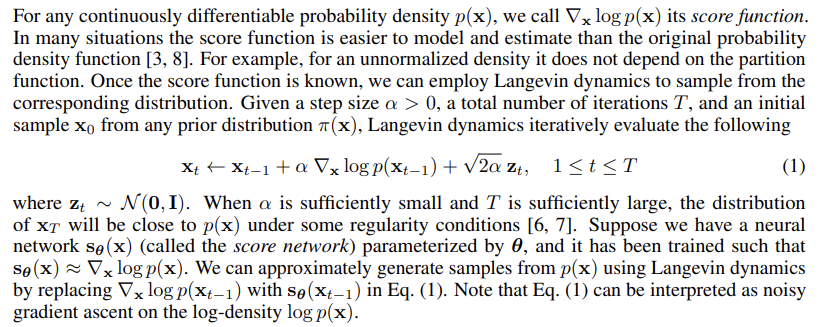
2.2. Score-based generative modeling


3. Choosing noise scales
Noise scales are critical for the success of NCSNs. As shown in [1], score networks trained with a single noise can never produce convincing samples for large images. Intuitively, high noise facilitates the estimation of score functions, but also leads to corrupted samples; while lower noise gives clean samples but makes score functions harder to estimate. One should therefore leverage different noise scales together to get the best of both worlds.
When the range of pixel values is [0, 1], the original work on NCSN [1] recommends choosing {σi} L i=1 as a geometric sequence where L = 10, σ1 = 1, and σL = 0.01. It is reasonable that the smallest noise scale σL = 0.01 << 1, because we sample from perturbed distributions with descending noise scales and we want to add low noise at the end. However, some important questions remain unanswered, which turn out to be critical to the success of NCSNs on high resolution images: (i) Is σ1 = 1 appropriate? If not, how should we adjust σ1 for different datasets? (ii) Is geometric progression a good choice? (iii) Is L = 10 good across different datasets? If not, how many noise scales are ideal?
Below we provide answers to the above questions, motivated by theoretical analyses on simple mathematical models. Our insights are effective for configuring score-based generative modeling in practice, as corroborated by experimental results in Section 6.
3.1. Initial noise scale


3.2. Other noise scales


3.3. Incorporating the noise information

handle a large number of noise scales (even continuous ones). As shown in Fig. 3 (detailed settings in Appendix B), it achieves similar training losses compared to the original noise conditioning approach in [1], and generate samples of better quality (see Appendix C.4).
4. Configuring annealed Langevin dynamics

5. Improving stability with moving average
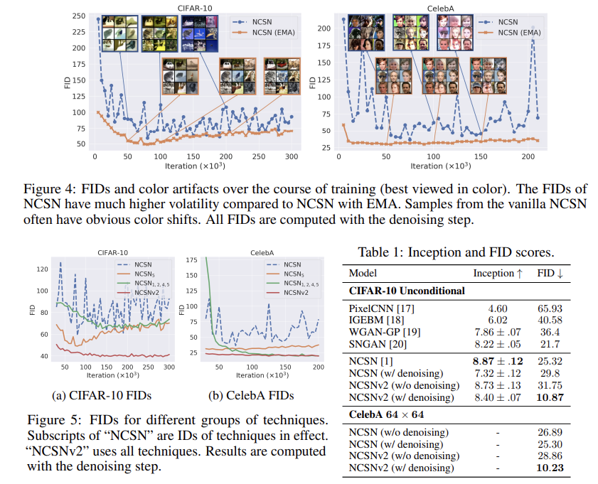
Unlike GANs, score-based generative models have one unified objective (Eq. (2)) and require no adversarial training. However, even though the loss function of NCSNs typically decreases steadily over the course of training, we observe that the generated image samples sometimes exhibit unstable visual quality, especially for images of larger resolutions. We empirically demonstrate this fact by training NCSNs on CIFAR-10 32 × 32 and CelebA [16] 64 × 64 following the settings of [1], which exemplifies typical behavior on other image datasets. We report FID scores [13] computed on 1000 samples every 5000 iterations. Results in Fig. 4 are computed with the denoising step, but results without the denoising step are similar (see Fig. 8 in Appendix C.1). As shown in Figs. 4 and 8, the FID scores for the vanilla NCSN often fluctuate significantly during training. Additionally, samples from the vanilla NCSN sometimes exhibit characteristic artifacts: image samples from the same checkpoint have strong tendency to have a common color shift. Moreover, samples are shifted towards different colors throughout training. We provide more samples in Appendix C.3 to manifest this artifact.
This issue can be easily fixed by exponential moving average (EMA). Specifically, let θi denote the parameters of an NCSN after the i-th training iteration, and θ' be an independent copy of the parameters. We update θ' with θ' ← mθ' + (1 − m)θi after each optimization step, where m is the momentum parameter and typically m = 0.999. When producing samples, we use sθ'(x, σ) instead of sθi(x, σ). As shown in Fig. 4, EMA can effectively stabilize FIDs, remove artifacts (more samples in Appendix C.3) and give better FID scores in most cases. Empirically, we observe the effectiveness of EMA is universal across a large number of different image datasets. As a result, we recommend the following rule of thumb:
Technique 5 (EMA). Apply exponential moving average to parameters when sampling.
6. Combining all techniques together
Employing Technique 1–5, we build NCSNs that can readily work across a large number of different datasets, including high resolution images that were previously out of reach with score-based generative modeling. Our modified model is named NCSNv2. For a complete description on experimental details and more results, please refer to Appendix B and C.
Quantitative results:
We consider CIFAR-10 32×32 and CelebA 64×64 where NCSN and NCSNv2 both produce reasonable samples. We report FIDs (lower is better) every 5000 iterations of training on 1000 samples and give results in Fig. 5 (with denoising) and Fig. 9 (without denoising, deferred to Appendix C.1). As shown in Figs. 5 and 9, we observe that the FID scores of NCSNv2 (with all techniques applied) are on average better than those of NCSN, and have much smaller variance over the course of training. Following [1], we select checkpoints with the smallest FIDs (on 1000 samples) encountered during training, and compute full FID and Inception scores on more samples from them. As shown by results in Table 1, NCSNv2 (w/ denoising) is able to significantly improve the FID scores of NCSN on both CIFAR-10 and CelebA, while bearing a slight loss of Inception scores on CIFAR-10. However, we note that Inception and FID scores have known issues [21, 22] and they should be interpreted with caution as they may not correlate with visual quality in the expected way. In particular, they can be sensitive to slight noise perturbations [23], as shown by the difference of scores with and without denoising in Table 1. To verify that NCSNv2 indeed generates better images than NCSN, we provide additional uncurated samples in Appendix C.4 for visual comparison.
Ablation studies:
We conduct ablation studies to isolate the contributions of different techniques. We partition all techniques into three groups: (i) Technique 5, (ii) Technique 1,2,4, and (iii) Technique 3, where different groups can be applied simultaneously. Technique 1,2 and 4 are grouped together because Technique 1 and 2 collectively determine the set of noise scales, and to sample from NCSNs trained with these noise scales we need Technique 4 to configure annealed Langevin dynamics properly. We test the performance of successively removing groups (iii), (ii), (i) from NCSNv2, and report results in Fig. 5 for sampling with denoising and in Fig. 9 (Appendix C.1) for sampling without denoising. All groups of techniques improve over the vanilla NCSN. Although the FID scores are not strictly increasing when removing (iii), (ii), and (i) progressively, we note that FIDs may not always correlate with sample quality well. In fact, we do observe decreasing sample quality by visual inspection (see Appendix C.4), and combining all techniques gives the best samples.
Towards higher resolution:
The original NCSN only succeeds at generating images of low resolution. In fact, [1] only tested it on MNIST 28 × 28 and CelebA/CIFAR-10 32 × 32. For slightly larger images such as CelebA 64 × 64, NCSN can generate images of consistent global structure, yet with strong color artifacts that are easily noticeable (see Fig. 4 and compare Fig. 10a with Fig. 10b). For images with resolutions beyond 96 × 96, NCSN will completely fail to produce samples with correct structure or color (see Fig. 7). All samples shown here are generated without the denoising step, but since σL is very small, they are visually indistinguishable from ones with the denoising step.
By combining Technique 1–5, NCSNv2 can work on images of much higher resolution. Note that we directly calculated the noise scales for training NCSNs, and computed the step size for annealed Langevin dynamics sampling without manual hyper-parameter tuning. The network architectures are the same across datasets, except that for ones with higher resolution we use more layers and more filters to ensure the receptive field and model capacity are large enough (see details in Appendix B.1). In Fig. 6 and 1, we show NCSNv2 is capable of generating high-fidelity image samples with resolutions ranging from 96 × 96 to 256 × 256. To show that this high sample quality is not a result of dataset memorization, we provide the loss curves for training/test, as well as nearest neighbors for samples in Appendix C.5. In addition, NCSNv2 can produce smooth interpolations between two given samples as in Fig. 6 (details in Appendix B.2), indicating the ability to learn generalizable image representations.

7. Conclusion
Motivated by both theoretical analyses and empirical observations, we propose a set of techniques to improve score-based generative models. Our techniques significantly improve the training and sampling processes, lead to better sample quality, and enable high-fidelity image generation at high resolutions. Although our techniques work well without manual tuning, we believe that the performance can be improved even more by fine-tuning various hyper-parameters. Future directions include theoretical understandings on the sample quality of score-based generative models, as well as alternative noise distributions to Gaussian perturbations.
B. Experimental details
B.1. Network architectures and hyperparameters
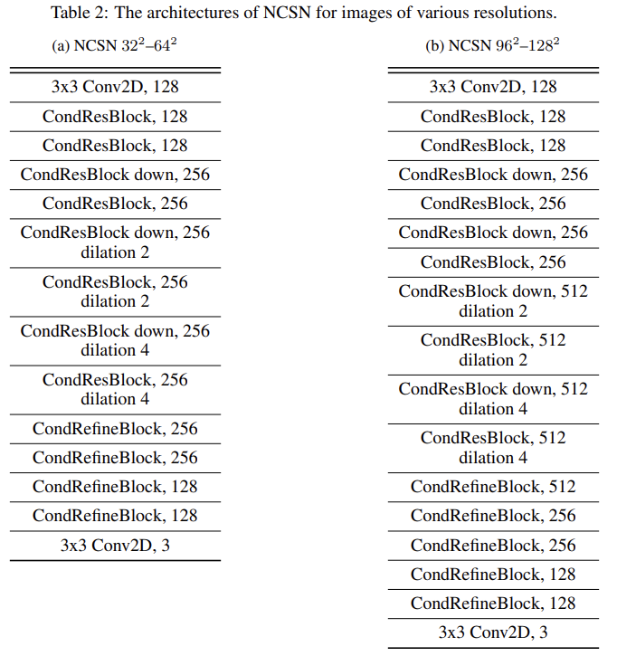
The original NCSN in [1] uses a network structure based on RefineNet [24]—a classical architecture for semantic segmentation. There are three major modifications to the original RefineNet in NCSN: (i) adding an enhanced version of conditional instance normalization (designed in [1] and named CondInstanceNorm++) for every convolutional layer; (ii) replacing max pooling with average pooling in RefineNet blocks; and (iii) using dilated convolutions in the ResNet backend of RefineNet. We use exactly the same architecture for NCSN experiments, but for NCSNv2 or any other architecture implementing Technique 3, we apply the following modifications: (i) setting the number of classes in CondInstanceNorm++ to 1 (which we name as InstanceNorm++); (ii) changing average pooling back to max pooling; and (iii) removing all normalization layers in RefineNet blocks. Here (ii) and (iii) do not affect the results much, but they are included because we hope to minimize the number of unnecessary changes to the standard RefineNet architecture (the original RefineNet blocks in [24] use max pooling and have no normalization layers). We name a ResNet block (with InstanceNorm++ instead of BatchNorm) “ResBlock”, and a RefineNet block “RefineBlock”. When CondInstanceNorm++ is added, we name them “CondResBlock” and “CondRefineBlock” respectively. We use the ELU activation function [25] throughout all architectures.
To ensure sufficient capacity and receptive fields, the network structures for images of different resolutions have different numbers of layers and filters. We summarize the architectures in Table 2 and Table 3.