6. Nonparametric Identification
https://www.bradyneal.com/causal-inference-course#course-textbook
In Section 4.4, we saw that satisfying the backdoor criterion is sufficient to give us identifiability, but is the backdoor criterion also necessary? In other words, is it possible to get identifiability without being able to block all backdoor paths?
As an example, consider that we have data generated according to the graph in Figure 6.1. We don't observe W in this data, so we can't block the backdoor path through W and the confounding association that flows along it. But we still need to identify the causal effect. I turns out that it is possible to identify the causal effect in this graph, using the frontdoor criterion.

We'll see the frontdoor criterion and corresponding adjustment in Section 6.1. Then we'll consider even more general identification in Section 6.2 when we introduce do-calculus. We'll conclude with graphical conditions for identifiability in Section 6.3.
6.1. Frontdoor Adjustment
The high-level intuition for why we can identify the causal effect of T on Y in the graph in Figure 6.1 (even when we can't adjust for the confounder W because it is unobserved) is as follows:
A mediator like M is very helpful; we can isolate the association that flows through M by focusing our statistical analysis on M, and the only association that flows through M is causal association (association flowing along directed paths from T to Y). We illustrate this intuition in Figure 6.2, where we depict only the causal association.

In this section, we will focus our analysis on M using a three step procedure.
1. Identify the causal effect of T on M.
2. Identify the causal effect of M on Y.
3. Combine the above steps to identify the causal effect of T on Y.

Step 1
First, we will identify the effect of T on M: P(m | do(t)). Because Y is a collider on the T - M path through W, it blocks that backdoor path. So there are no unblocked backdoor paths from T to M. This means that the only association that flows from T to M is the causal association that flows along the edge connecting them. Therefore, we have the following identification via the backdoor adjustment (Theorem 4.2, using the empty set as the adjustment set):

Step 2
Second, we will identify the effect of M on Y: P(y | do(m)). Because T blocks the backdoor path M ← T ← W → Y, we can simply adjust for T. Therefore, using the backdoor adjustment again, we have the following:

Step 3
Now that we know how changing T changes M (step 1) and how changing M changes Y (step 2), we can combine these two to get how changing T changes Y (through M):

The first factor on the right-hand side corresponds to setting T to t and observing the resulting value of M. The second factor corresponds to setting M to exactly the value m that resulted from setting T and then observing what value of Y results.
We must sum over m because P(m | do(t)) is probabilistic, so we must sum over its support. In other words, we must sum over all possible realizations m of the random variables whose distribution is P(M | do(t)).
If we then plug in Equations 6.1 and 6.2 into Equation 6.3, we get the frontdoor adjustment.

The causal graph we've been using (Figure 6.4) is an example of a simple graph that satisfies the frontdoor criterion.

To get the full definition, we must first define complete/full mediation: a set of variables M completely mediates the effect of T on Y if all causal (directed) paths from T to Y go through M.
We now give the general definition of the frontdoor criterion:

Although Equations 6.1 and 6.2 are straightforward applications of the backdoor adjustment, we hand-waved our way to Equation 6.3, which was key to the frontdoor adjustment (Theorem 6.1). We'll now walk through how to get Equation 6.3.
Proof. As usual, we start with the the truncated factorization, using the causal graph in Figure 6.4. From the Bayesian network factorization (Definition 3.1), we have the following:

Then, using the truncated factorization (Proposition 4.1), we remove the factor for T:

Next, we marginalize out w and m:

Even though we've removed all the do operators, recall that we are not done because W is unobserved. So we must also remove the w from the expression. This is where we have to get a bit creative.
We want to be able to combine P(y | w, m) and P(w) into a joint factor over both y and w so that we can marginalize out w. To do this, we need to get m behind the conditioning bar of the P(w) factor. This would be easy if we could just swap P(w) out for P(w | m) in Equation 6.8. The key thing to notice is that we actually can include m behind the conditioning bar if t were also there because T d-separates W from M in Figure 6.6. In math, this means that the following equality holds:


So how do we get t into this party? The usual trick of conditioning on it and marginalizing it out:

This matches the result stated in Theorem 6.1, so we've completed the derivation of the frontdoor adjustment without using the backdoor adjustment. However, we still need to show that Equation 6.3 is correct to justify step 3. To do that, all that's left is to recognize that these parts match Equation 6.1 and 6.2 and plug those in:

And we're done! We just needed to be a bit clever with our uses of d-separation and marginalization. Part of why we went through that proof is because we will prove the frontdoor adjustment using do-calculus in Section 6.2. This way you can easily compare a proof using the truncated factorization to a proof using do-calculus to prove the same result.
6.2. do-calculus
As we saw in the last section, it turns out that satisfying the backdoor criterion (Definition 4.1) isn't necessary to identify causal effects. For example, if the frontdoor criterion (Definition 6.1) is satisfied, that also gives us identifiability. This leads to the following questions: can we identify causal estimands when the associated causal graph satisfies neither the backdoor criterion nor the frontdoor criterion? If so, how? Pearl's do-calculus gives us the answer to these questions.
The do-calculus gives us tools to identify causal effects using the causal assumptions encoded in the causal graph. It will allow us to identify any causal estimand that is identifiable. More concretely, consider an arbitrary causal estimand P(Y | do(T = t), X = x), where Y is an arbitrary set of outcome variables, T is an arbitrary set of treatment variables, and X is an arbitrary (potentially empty) set of covariates that we want to chose how specific the causal effect we're looking at is. Note that this means we can use do-calculus to identify causal effects where there are multiple treatments and/or multiple outcomes.
In order to present the rules of do-calculus, we must define a bit of notation for augmented versions of the causal graph G. Let G_Xbar denote the graph that we get if we take G and remove all of the incoming edges to nodes in the set X; This is known as the manipulated graph.
Let G_Xunderbar denote the graph that we get if we take G and remove all of the outgoing edges from nodes in the set X. Think of parents as drawn above their children in the graph, so the var above X is cutting its incoming edges and the bar below X is cutting its outgoing edges. Combining these two we'll use G Xbar, Z underbar to denote the graph with the incoming edges to X and the outgoing edges from Z removed. We use ㅛG to denote d-separation in G.
do-calculus consists of just three rules:

We'll give intuition for each of them in terms of concepts we've already seen in this book.
Rule 1 Intuition
If we take Rule 1 and simply remove the intervention do(t), we get the following:

This is just what d-separation gives us under the Markov assumption; recall from Theorem 3.1 that d-separation in the graph implies conditional independence in P. This means that Rule 1 is simply a generalization of Theorem 3.1 to interventional distributions.
Rule 2 Intuition
Just as with Rule 1, we'll remove the intervention do(t) from Rule 2 and see what this reminds us of:

This is exactly what we do when we justify the backdoor adjustment (Theorem 4.2) using the backdoor criterion (Definition 4.1). Association is causation if the outcome Y and the treatment Z are d-separated by some set of variables that are conditioned on W. So rule 2 is a generalization of the backdoor adjustment to interventional distributions.
Rule 3 Intuition
-------------------- 이해 못 함 -------------------
Just as with the other two rules, we'll first remove the intervention do(t) to make thinking about this simpler:

To get the equality in this equation, it must be the case that removing the intervention do(z) (which is like taking the manipulated graph and reintroducing the edges going into Z) introduces no new association that can affect Y. Because do(z) removes the incoming edges to Z to give us Gzbar, the main association that we need to wory about is association flowing from Z to Y in Gzbar (causal association).
Therefore, you might expect that the condition that gives us the equality in Equation 6.23 is Y ㅛGzbar Z | W. However, we have to refine this a bit to prevent inducing association by conditioning on the descendants of collliders. Namely, Z could contain colliders in G, and W could contain descendants of these colliders. Therefore, to not induce new association through colliders in Z when we reintroduce the incoming edges to Z to get G, we must limit the set of manipulated nodes to these that are not ancestors of nodes in the conditioning set W: Z(W).
Rule 3는 무슨 말인지는 알겠는데, 그림이 안그려진다...
-------------------- 이해 못 함 -------------------
Completeness of do-calculus
Maybe there could exist causal estimands that are identifiable but that can't be identified using only the rules of do-calculus in Theorem 6.2. Fortunately, Shpitser and Pearl and Huang and Valtorta independently proved that this is not the case. They proved that do-calculus is complete, which means that these three rules are sufficient to identify all identifiable causal estimands. Because these proofs are constructive, they also admit algorithms that identify any causal estimand in polynomial time.
Nonparametric Identification
Note that all of this is about nonparametric identification; in other words, do-calculus tells us if we can identify a given causal estimand using only the causal assumptions encoded in the causal graph. If we introduce more assumptions about the distribution (e.g. linearity), we can identify more causal estimands. That would be known as parametric identification.
6.2.1. Application: Frontdoor Adjustment
Recall the simple graph we used that satisfies the frontdoor criterion (Figure 6.7), and recall the frontdoor adjustment:


At the end of Section 6.1, we saw a proof for the frontdoor adjustment using just the truncated factorization. To get an idea for how do-calculus works and the intuition we use in proofs that use it, we'll now do the frontdoor adjustment proof using the rules of do-calculus.
Proof.
Our goal is to identify P(y | do(t)). Because we have the intuition we described in Section 6.1 that the full mediator M will help us out, the first thing we'll do is introduce M into the equation via the marginalization trick:

Because the backdoor path from T to M in Figure 6.7 is blocked by the collider Y, all of the association that flows from T to M is causal, so we can apply Rule 2 to get the following:

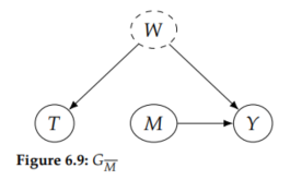
Now because M is a full mediator of the causal effect of T on Y, we should be able to replace P(y | do(t), m) with P(y | do(m)), but this will take two steps of do-calculus. To remove do(t), we'll need to use Rule 3, which requires that T have no causal effect on Y in the relevant graph. We can get to a graph like that by removing the edge from T to M (Figure 6.9); in do-calculus, we do this by using Rule 2 (in the opposite direction as before) to do(m). We can do this because the existing do(t) makes it so there are no backdoor paths from M to Y in G_Tbar (Figure 6.8).

Now, as we planned, we can remove the do(t) using Rule 3. We can use Rule 3 here because there is no causation flowing from T to Y in G_Mbar (Figure 6.9).


All that's left is to remove this last do-operator. As we discussed in Section 6.1, T blocks the only backdoor path from M to Y in the graph (Figure 6.10). This means, that if we can condition on T, we can get rid of this last do-operator. As usual, we do that by conditioning on and marginalizing out T. Rearranging a bit and using t' for the marginalization since t is already present:

Now, we can simply apply Rule 2, since T blocks the backdoor path from M to Y:

And finally, we can apply Rule 3 to remove the last do(m) because there is no causal effect of M on T (i.e. there is no directed path from M to T in the graph in (Figure 6.10).


6.3. Determining Identifiability from the Graph
It's nice to know that we can identify any causal estimand that is possible to identify using do-calculus, but this isn't as satisfying as knowing whether a causal estimand is identifiable by simply looking at the causal graph.
For example, the backdoor criterion (Definition 4.1) and the frontdoor criterion (Definition 6.1) gave us simple ways to know for sure that a causal estimand is identifiable. However, there are plenty of causal estimands that are identifiable, even though the corresponding causal graphs don't satisfy the backdoor or frontdoor criterion. More general graphical criteria exist that will tell us that these estimands are identifiable. We will discuss these more general graphical criteria for identifiability in this section.
Single Variable Intervention
When we care about causal effects of an intervention on a single variable, Tian and Pearl provide a relatively simple graphical criterion that is sufficient for identifiability: the unconfounded children criterion.

This criterion generalizes the backdoor criterion (Definition 4.1) and the frontdoor criterion (Definition 6.1). Like them, it is a sufficient condition for identifiability:

The intuition for unconfounded children criterion implies identifiability is similar to the intuition for the frontdoor criterion; if we can isolate all of the causal association flowing out of treatment along directed paths to Y, we have identifiability. To see this intuition, first, consider that all of the causal association from T must flow through its children. We can isolate this causal association if there is no confounding between T and any of its children. This isolation of all of the causal association is what gives us identifiability of the causal effect of T on any other node in the graph. This intuition might lead you to suspect that this criterion is necessary in the very specific case where the outcome set Y is all of the other variables in the graph other than T; it turns out that this is true. But this condition is not necessary if Y is smaller set than that.
To give you a more visual grasp of the intuition for why the unconfounded children criterion is sufficient for identification, we give an example graph in Figure 6.12. In Figure 6.12a, we visualize the flow of confounding association and causal association that flows in this graph. Then we depict the isolation of the causal association in that graph in Figure 6.12b.


Necessary Condition
The unconfounded children criterion is not necessary for identifiability, but it might aid your graphical intuition to have a necessary condition in mind. Here is one: For each backdoor path from T to any child M of T that is an ancestor of Y, it is possible to block that path. The intuition for this is that because the causal association that flows from T to Y must go through children of T that are ancestors of Y, to be able to isolate this causal association, the effect of T on these mediating children must be unconfounded. And a prerequisite to these T - M (parent-child) relationships being unconfounded is that any single backdoor path from T to M must be blockable (what we state in this condition).
Unfortunately, this condition is not sufficient. To see why, consider Figure 6.11. The backdoor path T ← W1 → W2 ← W3 → Y is blocked by the collider W2. However, conditioning on W2 unblocks the other backdoor path where W2 is a collider. Being able to block both paths individually does not mean we can block them both with a single conditioning set.
In sum, the unconfounded children criterion is sufficient but not necessary, and this related condition is necessary but not sufficient. Also, everything we've seen in this section so far is for a single variable intervention.
Necessary and Sufficient Conditions for Multiple Variable Interventions
Shpitser and Pearl [25] provide a necessary and sufficient criterion for identifiability of P(Y = y | do(T = t)) when Y and T are arbitrary sets of variables: the hedge criterion. However, this is outside the scope of this book, as it requires more complex objects such as hedges, C-trees, and other leafy objects. Moving further along, Shpitser and Pearl provide a necessary and sufficient criterion for the most general type of causal estimand: conditional causal effects, which take the form P(Y = y | do(T = t), X = x), where Y, T, and X are all arbitrary sets of variables.
