Synthetic Difference in Differences
https://arxiv.org/pdf/1812.09970
Abstract
We present a new estimator for causal effects with panel data that builds on insights behind the widely used difference in differences and synthetic control methods. Relative to these methods we find, both theoretically and empirically, that this “synthetic difference in differences” estimator has desirable robustness properties, and that it performs well in settings where the conventional estimators are commonly used in practice. We study the asymptotic behavior of the estimator when the systematic part of the outcome model includes latent unit factors interacted with latent time factors, and we present conditions for consistency and asymptotic normality.
1. Introduction
Researchers are often interested in evaluating the effects of policy changes using panel data, i.e., using repeated observations of units across time, in a setting where some units are exposed to the policy in some time periods but not others. These policy changes are frequently not random—neither across units of analysis, nor across time periods—and even unconfoundedness given observed covariates may not be credible (e.g., Imbens and Rubin [2015]). In the absence of exogenous variation researchers have focused on statistical models that connect observed data to unobserved counterfactuals. Many approaches have been developed for this setting but, in practice, a handful of methods are dominant in empirical work. As documented by Currie, Kleven, and Zwiers [2020], Difference in Differences (DID) methods have been widely used in applied economics over the last three decades; see also Ashenfelter and Card [1985], Bertrand, Duflo, and Mullainathan [2004], and Angrist and Pischke [2008]. More recently, Synthetic Control (SC) methods, introduced in a series of seminal papers by Abadie and coauthors [Abadie and Gardeazabal, 2003, Abadie, Diamond, and Hainmueller, 2010, 2015, Abadie and L’Hour, 2016], have emerged as an important alternative method for comparative case studies.
Currently these two strategies are often viewed as targeting different types of empirical applications. In general, DID methods are applied in cases where we have a substantial number of units that are exposed to the policy, and researchers are willing to make a “parallel trends” assumption which implies that we can adequately control for selection effects by accounting for additive unit-specific and time-specific fixed effects. In contrast, SC methods, introduced in a setting with only a single (or small number) of units exposed, seek to compensate for the lack of parallel trends by re-weighting units to match their pre-exposure trends.
In this paper, we argue that although the empirical settings where DID and SC methods are typically used differ, the fundamental assumptions that justify both methods are closely related. We then propose a new method, Synthetic Difference in Differences (SDID), that combines attractive features of both. Like SC, our method re-weights and matches pre-exposure trends to weaken the reliance on parallel trend type assumptions. Like DID, our method is invariant to additive unit-level shifts, and allows for valid large-panel inference. Theoretically, we establish consistency and asymptotic normality of our estimator. Empirically, we find that our method is competitive with (or dominates) DID in applications where DID methods have been used in the past, and likewise is competitive with (or dominates) SC in applications where SC methods have been used in the past.
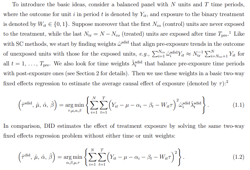
The use of weights in the SDID estimator effectively makes the two-way fixed effect regression “local,” in that it emphasizes (puts more weight on) units that on average are similar in terms of their past to the target (treated) units, and it emphasizes periods that are on average similar to the target (treated) periods.
This localization can bring two benefits relative to the standard DID estimator. Intuitively, using only similar units and similar periods makes the estimator more robust. For example, if one is interested in estimating the effect of anti-smoking legislation on California (Abadie, Diamond, and Hainmueller [2010]), or the effect of German reunification on West Germany (Abadie, Diamond, and Hainmueller [2015]), or the effect of the Mariel boatlift on Miami (Card [1990], Peri and Yasenov [2019]), it is natural to emphasize states, countries or cities that are similar to California, West Germany, or Miami respectively relative to states, countries or cities that are not. Perhaps less intuitively, the use of the weights can also improve the estimator’s precision by implicitly removing systematic (predictable) parts of the outcome. However, the latter is not guaranteed: If there is little systematic heterogeneity in outcomes by either units or time periods, the unequal weighting of units and time periods may worsen the precision of the estimators relative to the DID estimator.
Unit weights are designed so that the average outcome for the treated units is approximately parallel to the weighted average for control units. Time weights are designed so that the average post-treatment outcome for each of the control units differs by a constant from the weighted average of the pre-treatment outcomes for the same control units. Together, these weights make the DID strategy more plausible. This idea is not far from the current empirical practice. Raw data rarely exhibits parallel time trends for treated and control units, and researchers use different techniques, such as adjusting for covariates or selecting appropriate time periods to address this problem (e.g., Abadie [2005], Callaway and Sant’anna [2020]). Graphical evidence that is used to support the parallel trends assumption is then based on the adjusted data. SDID makes this process automatic and applies a similar logic to weighting both units and time periods, all while retaining statistical guarantees. From this point of view, SDID addresses pretesting concerns recently expressed in Roth [2018].
In comparison with the SDID estimator, the SC estimator omits the unit fixed effect and the time weights from the regression function:
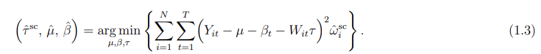
The argument for including time weights in the SDID estimator is the same as the argument for including the unit weights presented earlier: The time weight can both remove bias and improve precision by eliminating the role of time periods that are very different from the post-treatment periods. Similar to the argument for the use of weights, the argument for the inclusion of the unit fixed effects is twofold. First, by making the model more flexible, we strengthen its robustness properties. Second, as demonstrated in the application and simulations based on real data, these unit fixed effects often explain much of the variation in outcomes and can improve precision.
2. An Application
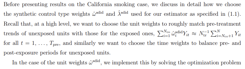
2.1. Implementing SDID
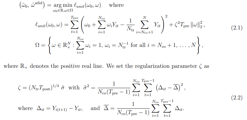
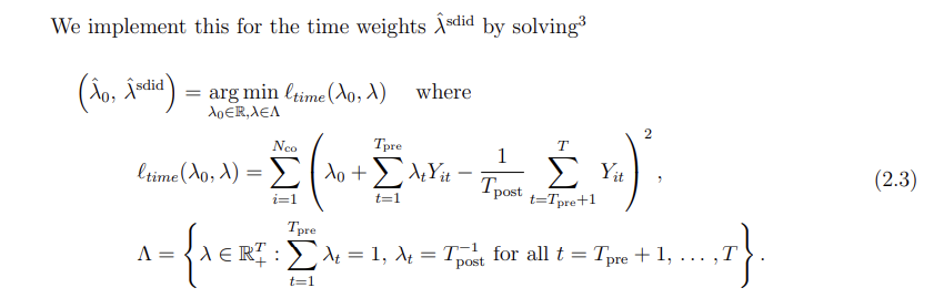
The main difference between (2.1) and (2.3) is that we use regularization for the former but not the latter. This choice is motivated by our formal results, and reflects the fact we allow for correlated observations within time periods for the same unit, but not across units within a time period, beyond what is captured by the systematic component of outcomes as represented by a latent factor model.
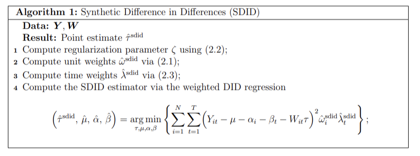
We summarize our procedure as Algorithm 1.4
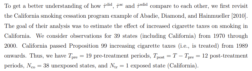
2.2. The California Smoking Cessation Program
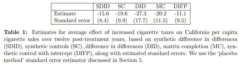
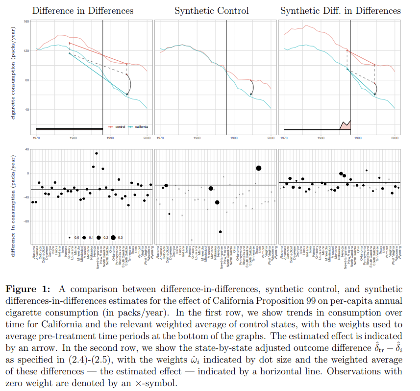
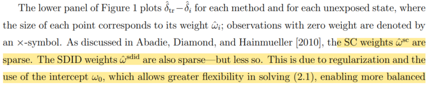
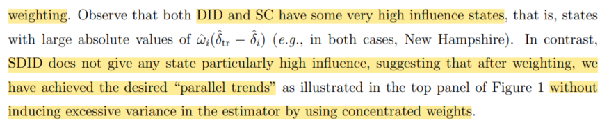
The top panel of Figure 1 illustrates how each method operates. As is well known [Ashenfelter and Card, 1985], DID relies on the assumption that cigarette sales in different states would have evolved in a parallel way absent the intervention. Here, pre-intervention trends are obviously not parallel, so the DID estimate should be considered suspect. In contrast, SC reweights the unexposed states so that the weighted of outcomes for these states match California pre-intervention as close as possible, and then attributes any post-intervention divergence of California from this weighted average to the intervention. What SDID does here is to re-weight the unexposed control units to make their time trend parallel (but not necessarily identical) to California pre-intervention, and then applies a DID analysis to this re-weighted panel. Moreover, because of the time weights, we only focus on a subset of the pre-intervention time periods when carrying out this last step. These time periods were selected so that the weighted average of historical outcomes predict average treatment period outcomes for control units, up to a constant. It is useful to contrast the data-driven SDID approach to selecting the time weights to both DID, where all pre-treatment periods are given equal weight, and to event studies where typically the last pre-treatment period is used as a comparison and so implicitly gets all the weight (e.g., Borusyak and Jaravel [2016], Freyaldenhoven et al. [2019]).
5. Large-Sample Inference
The asymptotic result from the previous section can be used to motivate practical methods for large-sample inference using SDID. Under appropriate conditions, the estimator is asymptotically normal and zero-centered; thus, if these conditions hold and we have a consistent estimator for its asymptotic variance Vτ , we can use conventional confidence intervals

to conduct asymptotically valid inference. In this section, we discuss three approaches to variance estimation for use in confidence intervals of this type.
(bootstrap & jackknife-based methods 생략... Third method - Placebo evaluation 사용할 예정)
Now, both the bootstrap and jackknife-based methods discussed so far are designed with the setting of Theorem 1 in mind, i.e., for large panels with many treated units. These methods may be less reliable when the number of treated units N_tr is small, and the jackknife is not even defined when N_tr = 1. However, many applications of synthetic controls have N_tr = 1, e.g., the California smoking application from Section 2. To this end, we consider a third variance estimator that is motivated by placebo evaluations as often considered in the literature on synthetic controls [Abadie, Diamond, and Hainmueller, 2010, 2015], and that can be applied with N_tr = 1. The main idea of such placebo evaluations is to consider the behavior of synthetic control estimation when we replace the unit that was exposed to the treatment with different units that were not exposed. Algorithm 4 builds on this idea, and uses placebo predictions using only the unexposed units to estimate the noise level, and then uses it to get Vτ^ and build confidence intervals as in (5.1). See Bottmer et al. [2021] for a discussion of the properties of such placebo variance estimators in small samples.
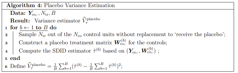
Validity of the placebo approach relies fundamentally on homoskedasticity across units, because if the exposed and unexposed units have different noise distributions then there is no way we can learn Vτ from unexposed units alone. We also note that non-parametric variance estimation for treatment effect estimators is in general impossible if we only have one treated unit, and so homoskedasticity across units is effectively a necessary assumption in order for inference to be possible here.
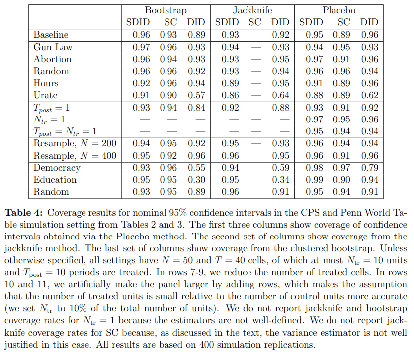
Table 4 shows the coverage rates for the experiments described in Section 3.1 and 3.2, using Gaussian confidence intervals (5.1) with variance estimates obtained as described above. In the case of the SDID estimation, the bootstrap estimator performs particularly well, yielding nearly nominal 95% coverage, while both placebo and jackknife variance estimates also deliver results that are close to the nominal 95% level. This is encouraging, and aligned with our previous observation that the SDID estimator appeared to have low bias. That being said, when assessing the performance of the placebo estimator, recall that the data in Section 3.1 was generated with noise that is both Gaussian and homoskedastic across units—which were assumptions that are both heavily used by the placebo estimator.
In contrast, we see that coverage rates for DID and SC can be relatively low, especially in cases with significant bias such as the setting with the state unemployment rate as the outcome. This is again in line with what one may have expected based on the distribution of the errors of each estimator as discussed in Section 3.1, e.g., in Figure 2: If the point estimates ˆτ from DID and SC are dominated by bias, then we should not expect confidence intervals that only focus on variance to achieve coverage.