5. Randomized Experiments

https://www.bradyneal.com/causal-inference-course#course-textbook

---

Randomized experiments are noticeably different from observational studies. In randomized experiments, the experimenter has complete control over the treatment assignment mechanism (how treatment is assigned). For example, in the most simple kind of randomized experiment, the experimenter randomly assigns (e.g. via coin toss) each participant to either the treatment group or the control group. This complete control over how treatment is chosen is what distinguished randomized experiments from observational studies. In this simple experimental setup, the treatment isn't a function of covariates at all! In contrast, in observational studies, the treatment is almost always a function of some covariate(s). This difference is key to whether or not confounding is present in our data.

 

In randomized experiments, association is causation. This is because randomized experiments are special in that they guarantee that there is no confounding. As a consequence, this allows us to measure the causal effect E[Y(1)] - E[Y(0)] via the associational difference E[Y | T=1] - E[Y | T=0].  

---

5.1. Comparability and Covariate Balance

Ideally, the treatment and control groups would be the same, in all aspects, except for treatment. This would mean they only differ in the treatment they receive (i.e. they are comparable). This would allow us to attribute any difference in the outcomes of the treatment and control groups to the treatment. 

 

Saying that these treatment groups are the same in everything other than their treatment and outcomes is the same as saying they have the same distribution of confounders. Because people often check for this property on observed variables (often what people mean by "covariates"), this concept is known as covariate balance. 

 

Randomization implies covariate balance, across all covariates, even unobserved ones. Intuitively, this is because the treatment is chosen at random, regardless of X, so the treatment and control groups should look very similar. The proof is simple. Because T is not at all determined by X (solely by a coin flip), T is independent of X. This means that P(X | T = 1) =d P(X). Similarly, it means P(X | T = 0) =d P(X). Therefore, we have P(X | T = 1) =d P(X | T = 0).

 

Although we have proven that randomization implies covariate balance, we have not proven that that covariate balance implies that association is causation.

 

We'll now prove that by showing that P(y | do(t)) = P(y | t). For the proof, the main property we utilize is that covariate balance implies X and T are independent.

 

Proof. First, let X be a sufficient adjustment set that potentially contains unobserved variables (randomization also balances unobserved covariates). Such an adjustment set must exist because we allow it to contain any variables, observed or unobserved. Then, we have the following from the backdoor adjustment (Theorem 4.2):

---

5.2. Exchangeability

Exchangeability (Assumption 2.1) gives us another perspective on why randomization makes causation equal to association. To see why, consider the following thought experiment. We decide an individual's treatment group using a random coin flip as follows: if the coin is heads, we assign the individual to the treatment group (T = 1), and if the coins is tails, we assign the individual to the control group (T = 0). If the groups are exchangeable, we could exchange these groups, and the average outcomes would remain the same. This is intuitively true if we chose the groups with a coin flip. Imagine simply swapping the meaning of "heads" and "tails" in this experiment. Would you expect that to change the results at all? No. This is why randomized experiments give us exchangeability.

 

Mean exchangeability is formally the following:

The "exchange" is when we go from Y(1) in the treatment group to Y(1) in the control group (Equation 5.8) and from Y(0) in the control group to Y(0) in the treatment group (Equation 5.9).

 

To see the proof of why association is causation in randomized experiments through the lens of exchangeability, recall the proof from Section 2.3.2. First, recall that Equation 5.8 means that both quantities in it are equal to the marginal expected outcome E[Y(1)] and, similarly, that Equation 5.9 means that both quantities in it are equal to the marginal expected outcome E[Y(0)]. Then, we have the following proof:

---

5.3. No Backdoor Paths

The final perspective that we'll look at to see why association is causation in randomized experiments is that of graphical causal models. In regular observational data, there is almost always confounding. 

 

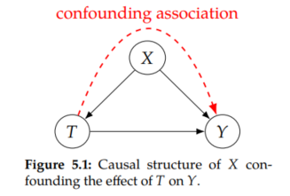
For example, in Figure 5.1, we see that X is a confounder of the effect of T on Y. Non-causal association flows along the backdoor path T ← X → Y. 

 

However, if we randomize T, something magical happens: T no longer has any causal parents, as we depict in Figure 5.2. This is because T is purely random. It doesn't depend on anything other than the output of a coin toss. Because T has no incoming edges, under randomization, there are no backdoor paths. So the empty set is a sufficient adjustment set. This means that all of the association that flows from T to Y is causal. 

 

We can identify P(Y | do(T = t)) by simply applying the backdoor adjustment (Theorem 4.2), adjusting for the empty set:

 

With that, we conclude our discussion of why association is causation in randomized experiments. 

---