[Lecture 9] (2/2) Policy Gradients and Actor Critics

https://storage.googleapis.com/deepmind-media/UCL%20x%20DeepMind%202021/Lecture%209-%20Policy%20gradients%20and%20actor%20critics.pdf

https://www.youtube.com/watch?v=y3oqOjHilio&list=PLqYmG7hTraZDVH599EItlEWsUOsJbAodm&index=9

---

What is and Actor Critics? Actor Critic is an agent that has an actor - a policy but it also has a value estimate - a critic. And we're going to talk about some concrete reasons for why you might want that. And what that could look like.

 

First, we're going to reduce variance. If you have any functional state b, we're calling it b for baseline, then the expectation of this b of function of state s times the gradient of the logarithm of pi will be zero for any b that does not depend on the action. 

 

Now we're going to use that to reduce variance and a very common choice for b is the value of your policy. We can estimate the value of the policy, we can just subtract that in the equation, and the expectation will remain unchanged. 

 

This is useful because it means that you can reduce the variance of the updates by picking this smartly. Because it will vary with states but it doesn't vary with actions. And this allows you to co-vary with q in such a way that you can reduce some of the variance in the updates.

 

So typically we just estimate this explicitly and then we can sample the q value as your Monte Carlo return. 

 

But since we have v now, we can also minimize variance further by instead picking a target that itself bootstraps. So instead of replacing q_pi with the full return from that moment onwards, we can also do the normal thing where we take on step or multiple steps and then bootstrap with a value. 

 

This will bias our gradient slightly potentially especially if you bootstrap after only one step, but it does reduce variance quite a bit. 

 

We'll talk more about techniques to reduce variance in the next lecture more generally and also especially when doing Off-policy learning which is going to be important for policy gradient algorithms in practice.

 

For now keep in mind that, this is a normal thing that people do all the time. They estimate value functions and these serve a double purpose. First, you can use them as a baseline, second, you can use them to bootstrap.

---

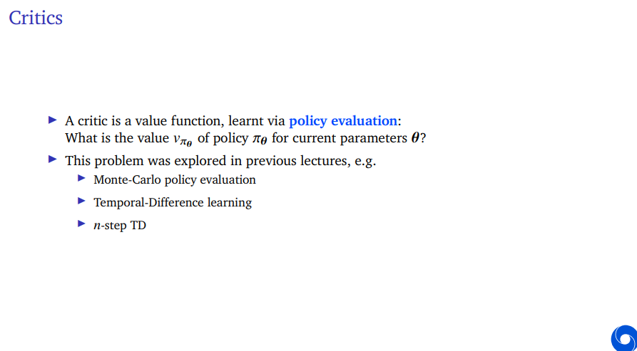
A critic is a value function learned via policy evaluation. We've considered Monte Carlo policy evaluation, Temporal Difference learning, and sub TD. You could use any of those in combination with the policy gradient algorithms to obtain an Actor Critic.

 

Then, the Actor Critic is simply, you update the parameters w of your value function with TD or Monte Carlo, and your update your policy parameters theta with policy gradients. then bootstrapping potentially.

---

Here is an example of a concrete algorithm which is a one-step Actor-Critic.

 

First, initialize w, theta and the state. So we are in some state S and then we're going to step through time. We are going to sample action according to our policy, we're going to sample a reward and a next state. 

 

We can then compute a one step TD error. Sometimes this one-step Temporal Difference error is called an advantage. Because you can argue that, this is in some sense, the advantage of taking the action or random instantiation of the advantage of taking the action that you took compared to all other actions. Because this temporal difference error does depend on the action that we took.

 

Then to update our critic, our value function. We can update the parameters thereof by adding a step size times your TD error times the gradient of your value function. 

 

And quite similarly we can update the policy parameters by adding a different step size which we here call alpha times the same temporal difference error times gradient of the logarithm of your policy. 

 

And this is a valid gradient update except for the fact that we're updating during the episode, and we're ignoring gamma to the power t term, which are two ways that you will slightly bias your policy gradient updates but they tend to work okay in practice. And they're just a little bit easier to use. You don't have to keep track of gamma to the power t term and in addition, by updating online, you can always update your policy already during the episode which can be beneficial if the episodes are really long. 

 

So this is a concrete instance of an Actor Critic algorithm where we have the Actor which is our policy with explicit parameters theta and we have our Critic which is the value function with parameters w which are both learned at the same time.

 

There are many variations of these algorithms and there's many ways to extend them in varous ways. But actually this main gist of this algorithm in some sense upderpins a lot of the current day algorithms that people use. So a lot of deep reinforcement learning in terms of applications uses algorithms that are remarkably similar to this one but just extended in various different ways. 

 

---

There's one thing to be particularly careful about which is that, bad policies might lead to bad data. Reinforcement learning is an active endeavor. The actions we take don't just influence our rewards but they also influence the data that you get. And that's a little bit different from supervised learning where we typically consider the data to be given. You can make bad classification mistakes or bad regression mistakes, but this won't influence the quality of the data that you can use to learn later.

 

In policy gradients, this can happen where you make a bad decision on how you update your parameters and all of a sudden, all of the data you get is garbage. 

---

So we have to be a little bit careful and one way to do that is, to increase stability by regularization and a popular method to do so is, to limit the difference between subsequent policies.

 

We want to make sure that we don't update the policy too much, because then, we might break it and all of a sudden your agent is just in the corner bumping his head against the wall and the data is not good enough to learn to do us anything else anymore.

 

So a popular thing here is, this is a difference between policies. Kullbeck-Leibler divergence, it's a distance between the old policy and the new policy. The nice thing about using a Kullbeck-Leibler divergence is that, it's differentiable. 

 

If you use this as a regularizer, it will try to keep you close. It will try to avoid changing your policy too much. The idea is to keep your policy from moving too much and this can avoid bad policy updates. 

---

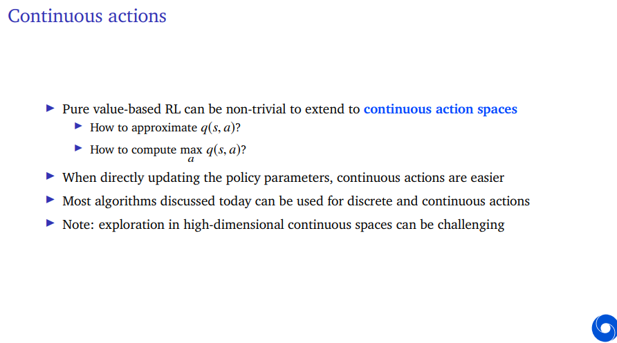
I'm going to talk about continuous action spaces and we can see how these algorithms are quite natural to extend to continuous action spaces.

 

So pure value-based RL can a little bit non-trivial to extend to continuous action spaces because how do we approximate the action value if the state space and the action space can both be continuous? If they can just be real-valued numbers or maybe even vectors. What if your action is a bunch of motor controls for a robot, which can have real-valued numbers? And how do we then compute if we could approximate this? how do we compute this maximization, how do we maximize our actions if we can't just select from a limited set? So there's a couple of practical problems if you would consider continuous actions.

 

But when we directly update the policy parameters, they're somewhat easier to deal with. And most algorithms, these policy gradient and actor-critic algorithms can be used for both discrete and continous actions. 

 

The only difference is how do we parameterize pi. How do I parameterize our policy.

 

Let's look at an example, but first before I do, I want to note that exploration in high-dimensional continuous spaces can be challenging. This has nothing to do with specific algorithms in some sense but if you have a very high dimensional space that you're searching in, it's hard. If your high dimensional space corresponds to actions that you're taking, exploration can be quite tricky. How do you pick an action from this high dimensional space? It is an interesting research problem and an interesting issue that we're going to have to deal with when we want to apply these algorithms at scale. 

---

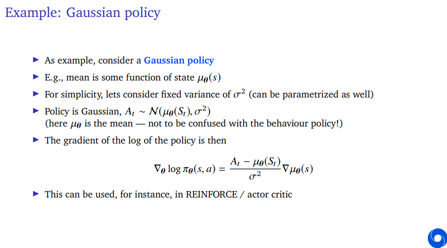
Let's consider a concrete instance of a continuous action algorithm. And to do so, we're going to parameterize our policy as a Gaussian policy which means, we're going to define some function of state which will represent the mean of our Gaussian and for simplicity, for now, we can keep it at that and we can say, there's some fixed variance. So for if this is a single dimensional policy, so we have a real-valued number and that will be our action. The mean will just be a number but it depends on state and it depends on our policy parameters theta and the variance will just be a number but we're going to consider it fixed. We could parameterize this as well. We could have policy parameters that are not just the mean of the Gaussian, but also the variance of the Gaussian. And then you could update them with policy gradients as well.

 

If we do that, the policy will pick an action according to the Gaussian distribution centered around that mean with the variance that we gave.

 

The policy itself is random because of this fixed variance which can be larger than zero, so the action you pick is a random quantity. 

 

Then, what does this grad log pi look like? What is the gradient of the logarithm of our policy? We can calculate that for the Gaussian policy. It looks like this where we see the action that we picked, and the difference between that action that we picked and the mean divided by our variance times the gradient of the mean.

 

So what does this mean? If we multiply this later on in a policy gradient algorithm with the return, if the return was positive, then this would update your mean towards the action that you took. If the return was negative, it would move away from the action you took. 

 

So we're going to sample this random action, and then depending on whether our signal from the critic or from the sampling the return depending on whether that's positive or negative, you would either move towards or away from the action you've taken.

 

And we can plug this into a policy gradient algorithm. 

---

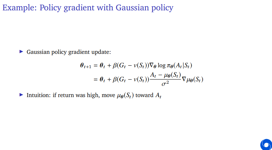
Let's say, we have a Monte Carlo return G, we're using that, we're not bootstrapping, we could also bootstrap but let's just say, we use Monte Carlo return, we have a baseline v, because you could also always use that, that doesn't change and then we just have this specific term which for the Gaussian policy. 

 

We can see that now instead of just looking at whether the return is high, we're looking, did we have a good surprise? because we're substracting baseline. The baseline does not change the expectation of the update, but it maybe makes it a little bit more interpretable. That is your return happens to be higher than you expected accroding to your value function, then you move the mean towards the action. That's what this would be doing. 

---

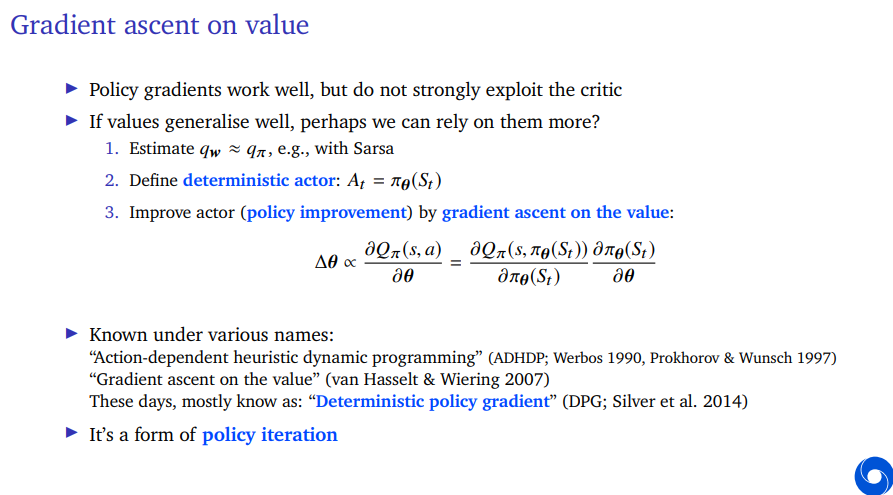
Now policy gradient algorithms they work really well and they underpin many of the current algorithms that people use in practice, but they don't actually exploit the critic all that strongly.

 

If you have a good critic, so if your value function is very accurate, can we maybe rely on it more? Can we do something else?

 

We're in the continuous action space. So we can estimate our action values with, for instance, SARSA. But we can also then define the deterministic actions. So the action here is either a real-valued number or it could even be a vector. So it could be a multi-dimensional output of this function. So our policy is now a deterministic policy. You're just plugging in your state and outcome is your actions that you're going to select.

 

Now, there's a thing you could do which is, if you can estimate the value of each action in each state which we can do by using SARSA or something like that, we can do policy improvements by moving the policy parameters in the direction of gradient ascent on the value quite directly. Because now we don't have to estimate this J function that we had before which was the expectation over all states and so on and so on. Now we're just saying, within this state, can we improve the value by taking the gradient with respect of this critic with respect to our policy parameters.

 

But how does this critic depend on our policy parameters? You can do the chain rule and we can look at how this value depends on our policy and then, how the policy depends on your parameters. This algorithm performs gradient ascent on the value and it's known under different names. 

 

Note that this is a form of policy iteration. So going back to dynamic programming, it's kind of an apt name in some sense, because we do have this notion here of doing policy evaluation and then using that to do policy improvement. But instead of doing a greedification step, we do a gradient step. We can do this gradient step because our policy is in this case, just outputting an action which is directly an input to this action value function and that means that we can just pass the gradient all the way through the action value function into the policy parameters. 

 

Of course, in practice, if you're going to estimate this quantity, if this is actually q_w rather than q_pi, because we don't know q_pi, if we plug in q_w, then this gradient could be biased and indeed that is an important thing if you want to make these policy gradient algorithms work. These deterministic policy gradient algorithms, you have to take some care you make sure that your critic estimates the values well. And that this gradient is well behaved. Because otherwise, it sometimes might just update your action into some weird situation, because the critic just thinks, if I make my action higher and higher and, I get more and more value which is not actually true but it might be what the critic thinks. So you have to be a little bit careful and maybe think about some stabilizing steps, regularization steps, if you want to use these algorithms. But then they can work quite well. 

---

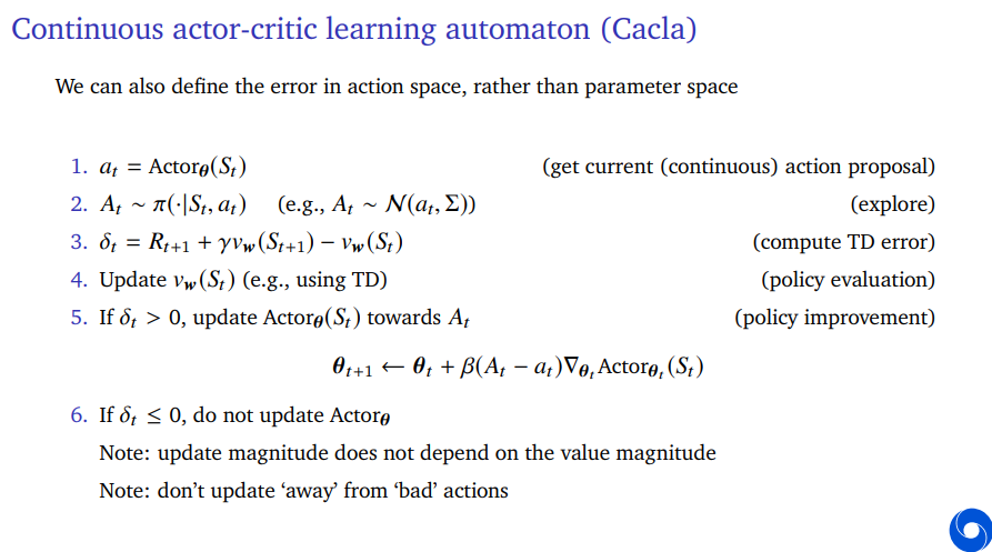
Now I want to talk about yet another algorithm. So why am I talking about different algorithms here, partially just to give you an intuition, and also to show you that there's actually many ways you can implement these algorithms, and many ways you can use them. And there's not one right way or one only way you could define an algorithm. So here's an algorithm called continuous active critical learning automation or Cacla. 

 

In this case, we're going to do something very similar to what we're doing before, but instead of defining the error in parameter space, we're going to define it in action space.

 

So how does the algorithm work? We're going to pick an action, this is just the output of an actor which is again deterministic. But now we're going to explicitly take into account exploration and we're going to sample for instance, from a Gaussian policy around the action. So this is similar to before, but here this is just purely considered an exploration step where we add a little bit of noise. But we could also add very deliberate noise. It doesn't have to be a Gaussian. It could be anything else you could just change your action in some way to deliberately pick a different action.

 

Then we can look at our Temporal Difference error similar to what we did for the Actor Critic. 

 

And then, we can update our value function using this Temporal Difference error or maybe we have a multi-step error, maybe we're doing Monte Carlo something else. We just define our Temporal Difference error in one way or the other and we update our value function as in normal Actor Critics.

 

But then to update the actor, we're going to do something slightly different. If the action value was positive, we update the actor towards the action that we took. So this is quite similar to what we saw before with the Gaussian policy. There is just a slight difference that we're not dividing by the variance of the exploration, and the other difference is that, the update does not depend on our values. There's no delta here. There's no TD error here. 

 

And the intuition behind this is that, maybe in order to decide how much you want to update your action, you don't want to look at how big the value is, because the value will be in completely different units from your actions. And if you're going to scale up your values or scale down your values or maybe in some states the values are just higher than others, then maybe your actor will be updated less or faster in some of those states than in others. Here instead, we're just going to look at, was the action a happy surprise? was it a good thing? was my Temporal Difference error positive? And if so, just update towards that action. So it's a slighly different algorithm. And if the Temporal Difference error is not positive, you simply don't update. That's another difference.

 

And why do we do that? The intuition is that, if you saw, let's say that you're close to optimal. And you have an actor that outputs very good actions, but you explore around that. Then actually most of the things you could explore around that would be bad. A lot of the actions apart from the one all the way at this top, we've done gradient ascent, we're at the top of some mountain in value space, and then we're considering an action that is a little bit away from that action, this will most likely be down. This will most likely be less good than the action that your current proposal from the actor. But that doesn't mean you should move in the other direction because then you'll just walk off the mountain in the other way. So instead of doing a gradient, here we're doing hill climbing. We're just looking at which actions work, and if they work, we move towards them. If they don't work, we don't know that moving away from them is a good idea. We don't know that, that will be up. We're just saying, if they're not good, we're not going to move. And the update of then therefore doesn't depend on the magnitude of the values. 

---

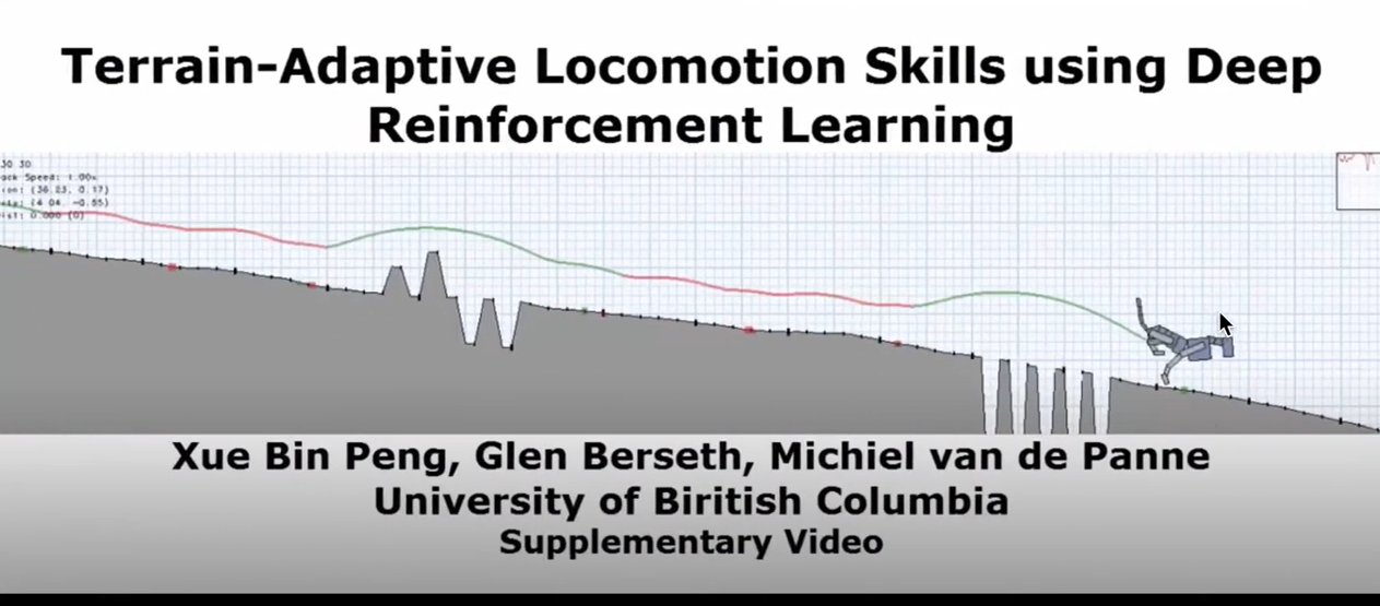
You can train these simulated animals running around. It could deal with several types of terrain. We can see that various different algorithms can be used to do things like this and to learn them.

 

And it's completely non-obvious how to do this yourself if you would have to write a policy that does this in continuous actions. That's actually very tricky.

 

Because it's a learning algorithm, it can also generalize to different body shapes, different terrains. This is benefit of learning that you can generalize in this way to things you haven't seen before.