Improved Denoising Diffusion Probabilistic Models

https://arxiv.org/pdf/2102.09672

---

Abstract

Denoising diffusion probabilistic models (DDPM) are a class of generative models which have recently been shown to produce excellent samples. We show that with a few simple modifications, DDPMs can also achieve competitive loglikelihoods while maintaining high sample quality. Additionally, we find that learning variances of the reverse diffusion process allows sampling with an order of magnitude fewer forward passes with a negligible difference in sample quality, which is important for the practical deployment of these models. We additionally use precision and recall to compare how well DDPMs and GANs cover the target distribution. Finally, we show that the sample quality and likelihood of these models scale smoothly with model capacity and training compute, making them easily scalable. We release our code at https://github.com/openai/improved-diffusion.

---

1. Introduction

Sohl-Dickstein et al. (2015) introduced diffusion probabilistic models, a class of generative models which match a data distribution by learning to reverse a gradual, multi-step noising process. More recently, Ho et al. (2020) showed an equivalence between denoising diffusion probabilistic models (DDPM) and score based generative models (Song & Ermon, 2019; 2020), which learn a gradient of the log-density of the data distribution using denoising score matching (Hyvarinen ¨ , 2005). It has recently been shown that this class of models can produce high-quality images (Ho et al., 2020; Song & Ermon, 2020; Jolicoeur-Martineau et al., 2020) and audio (Chen et al., 2020b; Kong et al., 2020), but it has yet to be shown that DDPMs can achieve loglikelihoods competitive with other likelihood-based models such as autoregressive models (van den Oord et al., 2016c) and VAEs (Kingma & Welling, 2013). This raises various questions, such as whether DDPMs are capable of capturing all the modes of a distribution. Furthermore, while Ho et al. (2020) showed extremely good results on the CIFAR-10 (Krizhevsky, 2009) and LSUN (Yu et al., 2015) datasets, it is unclear how well DDPMs scale to datasets with higher diversity such as ImageNet. Finally, while Chen et al. (2020b) found that DDPMs can efficiently generate audio using a small number of sampling steps, it has yet to be shown that the same is true for images.

 

In this paper, we show that DDPMs can achieve loglikelihoods competitive with other likelihood-based models, even on high-diversity datasets like ImageNet. To more tightly optimise the variational lower-bound (VLB), we learn the reverse process variances using a simple reparameterization and a hybrid learning objective that combines the VLB with the simplified objective from Ho et al. (2020).

 

We find surprisingly that, with our hybrid objective, our models obtain better log-likelihoods than those obtained by optimizing the log-likelihood directly, and discover that the latter objective has much more gradient noise during training. We show that a simple importance sampling technique reduces this noise and allows us to achieve better log-likelihoods than with the hybrid objective.

 

After incorporating learned variances into our model, we surprisingly discovered that we could sample in fewer steps from our models with very little change in sample quality. While DDPM (Ho et al., 2020) requires hundreds of forward passes to produce good samples, we can achieve good samples with as few as 50 forward passes, thus speeding up sampling for use in practical applications. In parallel to our work, Song et al. (2020a) develops a different approach to fast sampling, and we compare against their approach, DDIM, in our experiments.

 

While likelihood is a good metric to compare against other likelihood-based models, we also wanted to compare the distribution coverage of these models with GANs. We use the improved precision and recall metrics (Kynka¨anniemi ¨ et al., 2019) and discover that diffusion models achieve much higher recall for similar FID, suggesting that they do indeed cover a much larger portion of the target distribution.

 

Finally, since we expect machine learning models to consume more computational resources in the future, we evaluate the performance of these models as we increase model size and training compute. Similar to (Henighan et al., 2020), we observe trends that suggest predictable improvements in performance as we increase training compute.

---

2. Denoising Diffusion Probbabilistic Models

We briefly review the formulation of DDPMs from Ho et al. (2020). This formulation makes various simplifying assumptions, such as a fixed noising process q which adds diagonal Gaussian noise at each timestep. For a more general derivation, see Sohl-Dickstein et al. (2015).

---

2.1. Definitions

Given a data distribution x0 ∼ q(x0), we define a forward noising process q which produces latents x1 through xT by adding Gaussian noise at time t with variance βt ∈ (0, 1) as follows:

Given sufficiently large T and a well behaved schedule of βt, the latent xT is nearly an isotropic Gaussian distribution. Thus, if we know the exact reverse distribution q(xt−1|xt), we can sample xT ∼ N (0, I) and run the process in reverse to get a sample from q(x0). However, since q(xt−1|xt) depends on the entire data distribution, we approximate it using a neural network as follows:

The combination of q and p is a variational auto-encoder (Kingma & Welling, 2013), and we can write the variational lower bound (VLB) as follows:

Aside from L0, each term of Equation 4 is a KL divergence between two Gaussians, and can thus be evaluated in closed form. To evaluate L0 for images, we assume that each color component is divided into 256 bins, and we compute the probability of pθ(x0|x1) landing in the correct bin (which is tractable using the CDF of the Gaussian distribution). Also note that while LT does not depend on θ, it will be close to zero if the forward noising process adequately destroys the data distribution so that q(xT|x0) ≈ N(0, I).

 

As noted in (Ho et al., 2020), the noising process defined in Equation 2 allows us to sample an arbitrary step of the noised latents directly conditioned on the input x0. With αt := 1−βt and α¯t := summation t s=0 α_s, we can write the marginal

 

where ε ∼ N(0, I). Here, 1 − α¯t tells us the variance of the noise for an arbitrary timestep, and we could equivalently use this to define the noise schedule instead of βt.

 

Using Bayes theorem, one can calculate the posterior q(xt−1|xt, x0) in terms of β˜ t and µ˜t(xt, x0) which are defined as follows:

---

2.2. Training in Practice

The objective in Equation 4 is a sum of independent terms L_t−1, and Equation 9 provides an efficient way to sample from an arbitrary step of the forward noising process and estimate Lt−1 using the posterior (Equation 12) and prior (Equation 3). We can thus randomly sample t and use the expectation E_t,x0,ε [L_t−1] to estimate L_vlb. Ho et al. (2020) uniformly sample t for each image in each mini-batch.

 

There are many different ways to parameterize µθ(xt, t) in the prior. The most obvious option is to predict µθ(xt, t) directly with a neural network. Alternatively, the network could predict x0, and this output could be used in Equation 11 to produce µθ(xt, t). The network could also predict the noise ε and use Equations 9 and 11 to derive

Ho et al. (2020) found that predicting ε worked best, especially when combined with a reweighted loss function:

 

This objective can be seen as a reweighted form of Lvlb (without the terms affecting Σθ). The authors found that optimizing this reweighted objective resulted in much better sample quality than optimizing Lvlb directly, and explain this by drawing a connection to generative score matching (Song & Ermon, 2019; 2020).

 

One subtlety is that L_simple provides no learning signal for Σθ(xt, t). This is irrelevant, however, since Ho et al. (2020) achieved their best results by fixing the variance to σ 2 t I rather than learning it. They found that they achieve similar sample quality using either σ 2 t = βt or σ 2 t = β˜ t, which are the upper and lower bounds on the variance given by q(x0) being either isotropic Gaussian noise or a delta function, respectively.

---

3. Improving the Log-likelihood

While Ho et al. (2020) found that DDPMs can generate highfidelity samples according to FID (Heusel et al., 2017) and Inception Score (Salimans et al., 2016), they were unable to achieve competitive log-likelihoods with these models. Loglikelihood is a widely used metric in generative modeling, and it is generally believed that optimizing log-likelihood forces generative models to capture all of the modes of the data distribution (Razavi et al., 2019). Additionally, recent work (Henighan et al., 2020) has shown that small improvements in log-likelihood can have a dramatic impact on sample quality and learnt feature representations. Thus, it is important to explore why DDPMs seem to perform poorly on this metric, since this may suggest a fundamental shortcoming such as bad mode coverage. This section explores several modifications to the algorithm described in Section 2 that, when combined, allow DDPMs to achieve much better log-likelihoods on image datasets, suggesting that these models enjoy the same benefits as other likelihood-based generative models.

 

To study the effects of different modifications, we train fixed model architectures with fixed hyperparameters on the ImageNet 64 × 64 (van den Oord et al., 2016b) and CIFAR-10 (Krizhevsky, 2009) datasets. While CIFAR-10 has seen more usage for this class of models, we chose to study ImageNet 64 × 64 as well because it provides a good trade-off between diversity and resolution, allowing us to train models quickly without worrying about overfitting. Additionally, ImageNet 64×64 has been studied extensively in the context of generative modeling (van den Oord et al., 2016c; Menick & Kalchbrenner, 2018; Child et al., 2019; Roy et al., 2020), allowing us to compare DDPMs directly to many other generative models.

 

The setup from Ho et al. (2020) (optimizing L_simple while setting σ 2 t = βt and T = 1000) achieves a log-likelihood of 3.99 (bits/dim) on ImageNet 64 × 64 after 200K training iterations. We found in early experiments that we could get a boost in log-likelihood by increasing T from 1000 to 4000; with this change, the log-likelihood improves to 3.77. For the remainder of this section, we use T = 4000, but we explore this choice in Section 4.

---

3.1. Learning Σθ(xt, t)

In Ho et al. (2020), the authors set Σθ(xt, t) = σ 2 t I, where σt is not learned. Oddly, they found that fixing σ 2 t to βt yielded roughly the same sample quality as fixing it to β˜ t. Considering that βt and β˜ t represent two opposite extremes, it is reasonable to ask why this choice doesn’t affect samples. One clue is given by Figure 1, which shows that βt and β˜ t are almost equal except near t = 0, i.e. where the model is dealing with imperceptible details. Furthermore, as we increase the number of diffusion steps, βt and β˜ t seem to remain close to one another for more of the diffusion process. This suggests that, in the limit of infinite diffusion steps, the choice of σt might not matter at all for sample quality. In other words, as we add more diffusion steps, the model mean µθ(xt, t) determines the distribution much more than Σθ(xt, t).

 

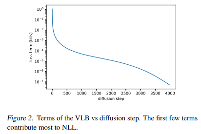
While the above argument suggests that fixing σt is a reasonable choice for the sake of sample quality, it says nothing about log-likelihood. In fact, Figure 2 shows that the first few steps of the diffusion process contribute the most to the variational lower bound. Thus, it seems likely that we could improve log-likelihood by using a better choice of Σθ(xt, t). To achieve this, we must learn Σθ(xt, t) without the instabilities encountered by Ho et al. (2020).

Since Figure 1 shows that the reasonable range for Σθ(xt, t) is very small, it would be hard for a neural network to predict Σθ(xt, t) directly, even in the log domain, as observed by Ho et al. (2020). Instead, we found it better to parameterize the variance as an interpolation between βt and β˜ t in the log domain. In particular, our model outputs a vector v containing one component per dimension, and we turn this output into variances as follows:

We did not apply any constraints on v, theoretically allowing the model to predict variances outside of the interpolated range. However, we did not observe the network doing this in practice, suggesting that the bounds for Σθ(xt, t) are indeed expressive enough.

 

Since L_simple doesn’t depend on Σθ(xt, t), we define a new hybrid objective:

For our experiments, we set λ = 0.001 to prevent L_vlb from overwhelming L_simple. Along this same line of reasoning, we also apply a stop-gradient to the µθ(xt, t) output for the L_vlb term. This way, L_vlb can guide Σθ(xt, t) while L_simple is still the main source of influence over µθ(xt, t). 

---

3.2. Improving the Noise Schedule

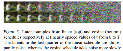
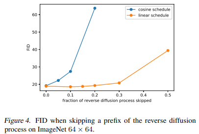
We found that while the linear noise schedule used in Ho et al. (2020) worked well for high resolution images, it was sub-optimal for images of resolution 64 × 64 and 32 × 32. In particular, the end of the forward noising process is too noisy, and so doesn’t contribute very much to sample quality. This can be seen visually in Figure 3. The result of this effect is studied in Figure 4, where we see that a model trained with the linear schedule does not get much worse (as measured by FID) when we skip up to 20% of the reverse diffusion process.

 

To address this problem, we construct a different noise schedule in terms of α¯t: 

To go from this definition to variances βt, we note that 

 

In practice, we clip βt to be no larger than 0.999 to prevent singularities at the end of the diffusion process near t = T.

 

Our cosine schedule is designed to have a linear drop-off of α¯t in the middle of the process, while changing very little near the extremes of t = 0 and t = T to prevent abrupt changes in noise level. Figure 5 shows how α¯t progresses for both schedules. We can see that the linear schedule from Ho et al. (2020) falls towards zero much faster, destroying information more quickly than necessary.

 

We use a small offset s to prevent  βt from being too small near t = 0, since we found that having tiny amounts of noise at the beginning of the process made it hard for the network to predict ε accurately enough. In particular, we selected s such that √ β0 was slightly smaller than the pixel bin size 1/127.5, which gives s = 0.008. We chose to use cos^2 in particular because it is a common mathematical function with the shape we were looking for. This choice was arbitrary, and we expect that many other functions with similar shapes would work as well.

---

3.3. Reducing Gradient Noise

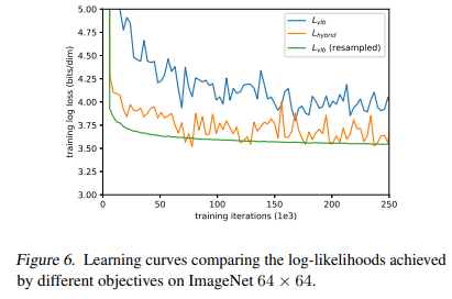
We expected to achieve the best log-likelihoods by optimizing L_vlb directly, rather than by optimizing L_hybrid. However, we were surprised to find that L_vlb was actually quite difficult to optimize in practice, at least on the diverse ImageNet 64×64 dataset. Figure 6 shows the learning curves for both L_vlb and L_hybrid. Both curves are noisy, but the hybrid objective clearly achieves better log-likelihoods on the training set given the same amount of training time.

 

We hypothesized that the gradient of L_vlb was much noisier than that of L_hybrid. We confirmed this by evaluating the gradient noise scales (McCandlish et al., 2018) for models trained with both objectives, as shown in Figure 7. Thus, we sought out a way to reduce the variance of L_vlb in order to optimize directly for log-likelihood.

 

Noting that different terms of L_vlb have greatly different magnitudes (Figure 2), we hypothesized that sampling t uniformly causes unnecessary noise in the L_vlb objective. To address this, we employ importance sampling:

Since E[L^2_t] is unknown beforehand and may change throughout training, we maintain a history of the previous 10 values for each loss term, and update this dynamically during training. At the beginning of training, we sample t uniformly until we draw 10 samples for every t ∈ [0, T −1]. With this importance  sampled objective, we are able to achieve our best log-likelihoods by optimizing L_vlb. This can be seen in Figure 6 as the L_vlb (resampled) curve. The figure also shows that the importance sampled objective is considerably less noisy than the original, uniformly sampled objective. We found that the importance sampling technique was not helpful when optimizing the less-noisy L_hybrid objective directly. 

---

3.4. Results and Ablations

In this section, we ablate the changes we have made to achieve better log-likelihoods. Table 1 summarizes the results of our ablations on ImageNet 64 × 64, and Table 2 shows them for CIFAR-10. We also trained our best ImageNet 64 × 64 models for 1.5M iterations, and report these results as well. L_vlb and L_hybrid were trained with learned sigmas using the parameterization from Section 3.1. For L_vlb, we used the resampling scheme from Section 3.3.

 

Based on our ablations, using L_hybrid and our cosine schedule improves log-likelihood while keeping similar FID as the baseline from Ho et al. (2020). Optimizing L_vlb further improves log-likelihood at the cost of a higher FID. We generally prefer to use L_hybrid over L_vlb as it gives a boost in likelihood without sacrificing sample quality.

 

In Table 3 we compare our best likelihood models against prior work, showing that these models are competitive with the best conventional methods in terms of log-likelihood.

---

4. Improving Sampling Speed

All of our models were trained with 4000 diffusion steps, and thus producing a single sample takes several minutes on a modern GPU. In this section, we explore how performance scales if we reduce the steps used during sampling, and find that our pre-trained L_hybrid models can produce high-quality samples with many fewer diffusion steps than they were trained with (without any fine-tuning). Reducing the steps in this way makes it possible to sample from our models in a number of seconds rather than minutes, and greatly improves the practical applicability of image DDPMs.

 

For a model trained with T diffusion steps, we would typically sample using the same sequence of t values (1, 2, ..., T) as used during training. However, it is also possible to sample using an arbitrary subsequence S of t values. Given the training noise schedule α¯t, for a given sequence S we can obtain the sampling noise schedule α¯St , which can be then used to obtain corresponding sampling variances

Now, since Σθ(xSt , St) is parameterized as a range between βSt and β˜ St , it will automatically be rescaled for the shorter diffusion process. We can thus compute p(xSt−1 |xSt ) as N (µθ(xSt , St), Σθ(xSt , St)).

 

To reduce the number of sampling steps from T to K, we use K evenly spaced real numbers between 1 and T (inclusive), and then round each resulting number to the nearest integer. In Figure 8, we evaluate FIDs for an L_hybrid model and an L_simple model that were trained with 4000 diffusion steps. steps, using 25, 50, 100, 200, 400, 1000, and 4000 sampling steps. We do this for both a fully-trained checkpoint, and a checkpoint mid-way through training. For CIFAR-10 we used 200K and 500K training iterations, and for ImageNet64 we used 500K and 1500K training iterations. We find that the L_simple models with fixed sigmas (with both the larger σ 2 t = βt and the smaller σ 2 t = β˜ t) suffer much more in sample quality when using a reduced number of sampling steps, whereas our L_hybrid model with learnt sigmas maintains high sample quality. With this model, 100 sampling steps is sufficient to achieve near-optimal FIDs for our fully trained models.

 

Parallel to our work, Song et al. (2020a) propose a fast sampling algorithm for DDPMs by producing a new implicit model that has the same marginal noise distributions, but deterministically maps noise to images. We include their algorithm, DDIM, in Figure 8, finding that DDIM produces better samples with fewer than 50 sampling steps, but worse samples when using 50 or more steps. Interestingly, DDIM performs worse at the start of training, but closes the gap to other samplers as training continues. We found that our striding technique drastically reduced performance of DDIM, so our DDIM results instead use the constant striding1 from Song et al. (2020a), wherein the final timestep is T − T /K + 1 rather than T. The other samplers performed slightly better with our striding.

---

5. Comparison to GANs

While likelihood is a good proxy for mode-coverage, it is difficult to compare to GANs with this metric. Instead, we turn to precision and recall (Kynka¨anniemi et al. ¨ , 2019). Since it is common in the GAN literature to train class-conditional models, we do the same for this experiment. To make our models class-conditional, we inject class information through the same pathway as the timestep t. In particular, we add a class embedding vi to the timestep embedding et, and pass this embedding to residual blocks throughout the model. We train using the L_hybrid objective and use 250 sampling steps. We train two models: a ”small” model with 100M parameters for 1.7M training steps, and a larger model with 270 million parameters for 250K iterations. We train one BigGAN-deep model with 100M parameters across the generator and discriminator.

 

When computing metrics for this task, we generated 50K samples (rather than 10K) to be directly comparable to other works.2 This is the only ImageNet 64 × 64 FID we report that was computed using 50K samples. For FID, the reference distribution features were computed over the full training set, following (Brock et al., 2018).

 

Figure 9 shows our samples from the larger model, and Table 4 summarizes our results. We find that BigGANdeep outperforms our smaller model in terms of FID, but struggles in terms of recall. This suggests that diffusion models are better at covering the modes of the distribution than comparable GANs.

---

6. Scaling Model Size

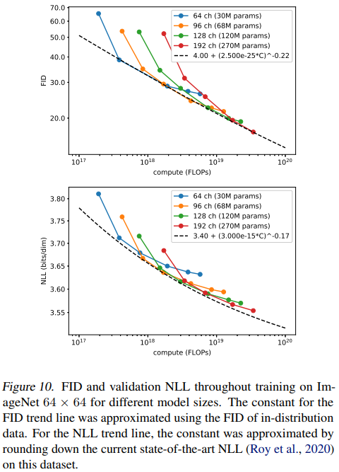
In the previous sections, we showed algorithmic changes that improved log-likelihood and FID without changing the amount of training compute. However, a trend in modern machine learning is that larger models and more training time tend to improve model performance (Kaplan et al., 2020; Chen et al., 2020a; Brown et al., 2020). Given this observation, we investigate how FID and NLL scale as a function of training compute. Our results, while preliminary, suggest that DDPMs improve in a predictable way as training compute increases.

 

To measure how performance scales with training compute, we train four different models on ImageNet 64 × 64 with the L_hybrid objective described in Section 3.1. To change model capacity, we apply a depth multiplier across all layers, such that the first layer has either 64, 96, 128, or 192 channels. Note that our previous experiments used 128 channels in the first layer. Since the depth of each layer affects the scale of the initial weights, we scale the Adam (Kingma & Ba, 2014) learning rate for each model by 1/ √ channel multiplier, such that the 128 channel model has a learning rate of 0.0001 (as in our other experiments).

 

Figure 10 shows how FID and NLL improve relative to theoretical training compute.3 The FID curve looks approximately linear on a log-log plot, suggesting that FID scales according to a power law (plotted as the black dashed line). The NLL curve does not fit a power law as cleanly, suggesting that validation NLL scales in a less-favorable manner than FID. This could be caused by a variety of factors, such as 1) an unexpectedly high irreducible loss (Henighan et al., 2020) for this type of diffusion model, or 2) the model overfitting to the training distribution. We also note that these models do not achieve optimal log-likelihoods in general because they were trained with our L_hybrid objective and not directly with L_vlb to keep both good log-likelihoods and sample quality.

---

7. Related Work

Chen et al. (2020b) and Kong et al. (2020) are two recent works that use DDPMs to produce high fidelity audio conditioned on mel-spectrograms. Concurrent to our work, Chen et al. (2020b) use a combination of improved schedule and L1 loss to allow sampling with fewer steps with very little reduction in sample quality. However, compared to our unconditional image generation task, their generative task has a strong input conditioning signal provided by the melspectrograms, and we hypothesize that this makes it easier to sample with fewer diffusion steps.

 

Jolicoeur-Martineau et al. (2020) explored score matching in the image domain, and constructed an adversarial training objective to produce better x0 predictions. However, they found that choosing a better network architecture removed the need for this adversarial objective, suggesting that the adversarial objective is not necessary for powerful generative modeling.

 

Parallel to our work, Song et al. (2020a) and Song et al. (2020b) propose fast sampling algorithms for models trained with the DDPM objective by leveraging different sampling processes. Song et al. (2020a) does this by deriving an implicit generative model that has the same marginal noise distributions as DDPMs while deterministically mapping noise to images. Song et al. (2020b) model the diffusion process as the discretization of a continuous SDE, and observe that there exists an ODE that corresponds to sampling from the reverse SDE. By varying the numerical precision of an ODE solver, they can sample with fewer function evaluations. However, they note that this technique obtains worse samples than ancestral sampling when used directly, and only achieves better FID when combined with Langevin corrector steps. This in turn requires hand-tuning of a signal-to-noise ratio for the Langevin steps. Our method allows fast sampling directly from the ancestral process, which removes the needs for extra hyperparameters.

 

Also in parallel, Gao et al. (2020) develops a diffusion model with reverse diffusion steps modeled by an energy-based model. A potential implication of this approach is that fewer diffusion steps should be needed to achieve good samples.

---

8. Conclusion

We have shown that, with a few modifications, DDPMs can sample much faster and achieve better log-likelihoods with little impact on sample quality. The likelihood is improved by learning Σθ using our parameterization and L_hybrid objective. This brings the likelihood of these models much closer to other likelihood-based models. We surprisingly discover that this change also allows sampling from these models with many fewer steps.

 

We have also found that DDPMs can match the sample quality of GANs while achieving much better mode coverage as measured by recall. Furthermore, we have investigated how DDPMs scale with the amount of available training compute, and found that more training compute trivially leads to better sample quality and log-likelihood.

 

The combination of these results makes DDPMs an attractive choice for generative modeling, since they combine good log-likelihoods, high-quality samples, and reasonably fast sampling with a well-grounded, stationary training objective that scales easily with training compute. These results indicate that DDPMs are a promising direction for future research.

---