-
Diffusion Models Beat GANs on Image Synthesis*Generative Model/Diffusion 2024. 8. 21. 02:34
https://arxiv.org/pdf/2105.05233
Abstract
We show that diffusion models can achieve image sample quality superior to the current state-of-the-art generative models. We achieve this on unconditional image synthesis by finding a better architecture through a series of ablations. For conditional image synthesis, we further improve sample quality with classifier guidance: a simple, compute-efficient method for trading off diversity for fidelity using gradients from a classifier. We achieve an FID of 2.97 on ImageNet 128×128, 4.59 on ImageNet 256×256, and 7.72 on ImageNet 512×512, and we match BigGAN-deep even with as few as 25 forward passes per sample, all while maintaining better coverage of the distribution. Finally, we find that classifier guidance combines well with upsampling diffusion models, further improving FID to 3.94 on ImageNet 256×256 and 3.85 on ImageNet 512×512. We release our code at https://github.com/openai/guided-diffusion.
1. Introduction

Over the past few years, generative models have gained the ability to generate human-like natural language [6], infinite high-quality synthetic images [5, 28, 51] and highly diverse human speech and music [64, 13]. These models can be used in a variety of ways, such as generating images from text prompts [72, 50] or learning useful feature representations [14, 7]. While these models are already capable of producing realistic images and sound, there is still much room for improvement beyond the current state-of-the-art, and better generative models could have wide-ranging impacts on graphic design, games, music production, and countless other fields.
GANs [19] currently hold the state-of-the-art on most image generation tasks [5, 68, 28] as measured by sample quality metrics such as FID [23], Inception Score [54] and Precision [32]. However, some of these metrics do not fully capture diversity, and it has been shown that GANs capture less diversity than state-of-the-art likelihood-based models [51, 43, 42]. Furthermore, GANs are often difficult to train, collapsing without carefully selected hyperparameters and regularizers [5, 41, 4].
While GANs hold the state-of-the-art, their drawbacks make them difficult to scale and apply to new domains. As a result, much work has been done to achieve GAN-like sample quality with likelihood-based models [51, 25, 42, 9]. While these models capture more diversity and are typically easier to scale and train than GANs, they still fall short in terms of visual sample quality. Furthermore, except for VAEs, sampling from these models is slower than GANs in terms of wall-clock time.
Diffusion models are a class of likelihood-based models which have recently been shown to produce high-quality images [56, 59, 25] while offering desirable properties such as distribution coverage, a stationary training objective, and easy scalability. These models generate samples by gradually removing noise from a signal, and their training objective can be expressed as a reweighted variational lower-bound [25]. This class of models already holds the state-of-the-art [60] on CIFAR-10 [31], but still lags behind GANs on difficult generation datasets like LSUN and ImageNet. Nichol and Dhariwal [43] found that these models improve reliably with increased compute, and can produce high-quality samples even on the difficult ImageNet 256×256 dataset using an upsampling stack. However, the FID of this model is still not competitive with BigGAN-deep [5], the current state-of-the-art on this dataset.
We hypothesize that the gap between diffusion models and GANs stems from at least two factors: first, that the model architectures used by recent GAN literature have been heavily explored and refined; second, that GANs are able to trade off diversity for fidelity, producing high quality samples but not covering the whole distribution. We aim to bring these benefits to diffusion models, first by improving model architecture and then by devising a scheme for trading off diversity for fidelity. With these improvements, we achieve a new state-of-the-art, surpassing GANs on several different metrics and datasets.
The rest of the paper is organized as follows. In Section 2, we give a brief background of diffusion models based on Ho et al. [25] and the improvements from Nichol and Dhariwal [43] and Song et al. [57], and we describe our evaluation setup. In Section 3, we introduce simple architecture improvements that give a substantial boost to FID. In Section 4, we describe a method for using gradients from a classifier to guide a diffusion model during sampling. We find that a single hyperparameter, the scale of the classifier gradients, can be tuned to trade off diversity for fidelity, and we can increase this gradient scale factor by an order of magnitude without obtaining adversarial examples [61]. Finally, in Section 5 we show that models with our improved architecture achieve state-of-the-art on unconditional image synthesis tasks, and with classifier guidance achieve state-of-the-art on conditional image synthesis. When using classifier guidance, we find that we can sample with as few as 25 forward passes while maintaining FIDs comparable to BigGAN. We also compare our improved models to upsampling stacks, finding that the two approaches give complementary improvements and that combining them gives the best results on ImageNet 256×256 and 512×512
2. Background
In this section, we provide a brief overview of diffusion models. For a more detailed mathematical description, we refer the reader to Appendix B.
On a high level, diffusion models sample from a distribution by reversing a gradual noising process. In particular, sampling starts with noise xT and produces gradually less-noisy samples xT −1, xT −2, ... until reaching a final sample x0. Each timestep t corresponds to a certain noise level, and xt can be thought of as a mixture of a signal x0 with some noise ε where the signal to noise ratio is determined by the timestep t. For the remainder of this paper, we assume that the noise ε is drawn from a diagonal Gaussian distribution, which works well for natural images and simplifies various derivations.
A diffusion model learns to produce a slightly more “denoised” xt−1 from xt. Ho et al. [25] parameterize this model as a function εθ(xt, t) which predicts the noise component of a noisy sample xt. To train these models, each sample in a minibatch is produced by randomly drawing a data sample x0, a timestep t, and noise ε , which together give rise to a noised sample xt (Equation 17). The training objective is then || εθ(xt, t) − ε ||2 , i.e. a simple mean-squared error loss between the true noise and the predicted noise (Equation 26).
It is not immediately obvious how to sample from a noise predictor εθ(xt, t). Recall that diffusion sampling proceeds by repeatedly predicting xt−1 from xt, starting from xT . Ho et al. [25] show that, under reasonable assumptions, we can model the distribution pθ(xt−1|xt) of xt−1 given xt as a diagonal Gaussian N (xt−1; µθ(xt, t), Σθ(xt, t)), where the mean µθ(xt, t) can be calculated as a function of ε θ(xt, t) (Equation 27). The variance Σθ(xt, t) of this Gaussian distribution can be fixed to a known constant [25] or learned with a separate neural network head [43], and both approaches yield high-quality samples when the total number of diffusion steps T is large enough.
Ho et al. [25] observe that the simple mean-sqaured error objective, L_simple, works better in practice than the actual variational lower bound L_vlb that can be derived from interpreting the denoising diffusion model as a VAE. They also note that training with this objective and using their corresponding sampling procedure is equivalent to the denoising score matching model from Song and Ermon [58], who use Langevin dynamics to sample from a denoising model trained with multiple noise levels to produce high quality image samples. We often use “diffusion models” as shorthand to refer to both classes of models.
2.1. Improvements
Following the breakthrough work of Song and Ermon [58] and Ho et al. [25], several recent papers have proposed improvements to diffusion models. Here we describe a few of these improvements, which we employ for our models.
Nichol and Dhariwal [43] find that fixing the variance Σθ(xt, t) to a constant as done in Ho et al. [25] is sub-optimal for sampling with fewer diffusion steps, and propose to parameterize Σθ(xt, t) as a neural network whose output v is interpolated as:

Here, βt and β˜ t (Equation 19) are the variances in Ho et al. [25] corresponding to upper and lower bounds for the reverse process variances. Additionally, Nichol and Dhariwal [43] propose a hybrid objective for training both εθ(xt, t) and Σθ(xt, t) using the weighted sum L_simple + λL_vlb. Learning the reverse process variances with their hybrid objective allows sampling with fewer steps without much drop in sample quality. We adopt this objective and parameterization, and use it throughout our experiments.
Song et al. [57] propose DDIM, which formulates an alternative non-Markovian noising process that has the same forward marginals as DDPM, but allows producing different reverse samplers by changing the variance of the reverse noise. By setting this noise to 0, they provide a way to turn any model εθ(xt, t) into a deterministic mapping from latents to images, and find that this provides an alternative way to sample with fewer steps. We adopt this sampling approach when using fewer than 50 sampling steps, since Nichol and Dhariwal [43] found it to be beneficial in this regime.
2.2. Sample Quality Metrics
For comparing sample quality across models, we perform quantitative evaluations using the following metrics. While these metrics are often used in practice and correspond well with human judgement, they are not a perfect proxy, and finding better metrics for sample quality evaluation is still an open problem.
Inception Score (IS) was proposed by Salimans et al. [54], and it measures how well a model captures the full ImageNet class distribution while still producing individual samples that are convincing examples of a single class. One drawback of this metric is that it does not reward covering the whole distribution or capturing diversity within a class, and models which memorize a small subset of the full dataset will still have high IS [3]. To better capture diversity than IS, Fréchet Inception Distance (FID) was proposed by Heusel et al. [23], who argued that it is more consistent with human judgement than Inception Score. FID provides a symmetric measure of the distance between two image distributions in the Inception-V3 [62] latent space. Recently, sFID was proposed by Nash et al. [42] as a version of FID that uses spatial features rather than the standard pooled features. They find that this metric better captures spatial relationships, rewarding image distributions with coherent high-level structure. Finally, Kynkäänniemi et al. [32] proposed Improved Precision and Recall metrics to separately measure sample fidelity as the fraction of model samples which fall into the data manifold (precision), and diversity as the fraction of data samples which fall into the sample manifold (recall).
We use FID as our default metric for overall sample quality comparisons as it captures both diversity and fidelity and has been the de facto standard metric for state-of-the-art generative modeling work [27, 28, 5, 25]. We use Precision or IS to measure fidelity, and Recall to measure diversity or distribution coverage. When comparing against other methods, we re-compute these metrics using public samples or models whenever possible. This is for two reasons: first, some papers [27, 28, 25] compare against arbitrary subsets of the training set which are not readily available; and second, subtle implementation differences can affect the resulting FID values [45]. To ensure consistent comparisons, we use the entire training set as the reference batch [23, 5], and evaluate metrics for all models using the same codebase.
3. Architecture Improvements
In this section we conduct several architecture ablations to find the model architecture that provides the best sample quality for diffusion models.
Ho et al. [25] introduced the UNet architecture for diffusion models, which Jolicoeur-Martineau et al. [26] found to substantially improve sample quality over the previous architectures [58, 33] used for denoising score matching. The UNet model uses a stack of residual layers and downsampling convolutions, followed by a stack of residual layers with upsampling colvolutions, with skip connections connecting the layers with the same spatial size. In addition, they use a global attention layer at the 16×16 resolution with a single head, and add a projection of the timestep embedding into each residual block. Song et al. [60] found that further changes to the UNet architecture improved performance on the CIFAR-10 [31] and CelebA-64 [34] datasets. We show the same result on ImageNet 128×128, finding that architecture can indeed give a substantial boost to sample quality on much larger and more diverse datasets at a higher resolution.
We explore the following architectural changes:
• Increasing depth versus width, holding model size relatively constant.
• Increasing the number of attention heads.
• Using attention at 32×32, 16×16, and 8×8 resolutions rather than only at 16×16.
• Using the BigGAN [5] residual block for upsampling and downsampling the activations, following [60].
• Rescaling residual connections with 1/√2, following [60, 27, 28].
For all comparisons in this section, we train models on ImageNet 128×128 with batch size 256, and sample using 250 sampling steps. We train models with the above architecture changes and compare them on FID, evaluated at two different points of training, in Table 1. Aside from rescaling residual connections, all of the other modifications improve performance and have a positive compounding effect. We observe in Figure 2 that while increased depth helps performance, it increases training time and takes longer to reach the same performance as a wider model, so we opt not to use this change in further experiments.
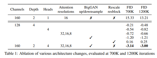
We also study other attention configurations that better match the Transformer architecture [66]. To this end, we experimented with either fixing attention heads to a constant, or fixing the number of channels per head. For the rest of the architecture, we use 128 base channels, 2 residual blocks per resolution, multi-resolution attention, and BigGAN up/downsampling, and we train the models for 700K iterations. Table 2 shows our results, indicating that more heads or fewer channels per head improves FID. In Figure 2, we see 64 channels is best for wall-clock time, so we opt to use 64 channels per head as our default. We note that this choice also better matches modern transformer architectures, and is on par with our other configurations in terms of final FID.


3.1. Adaptive Group Normalization
We also experiment with a layer [43] that we refer to as adaptive group normalization (AdaGN), which incorporates the timestep and class embedding into each residual block after a group normalization operation [69], similar to adaptive instance norm [27] and FiLM [48]. We define this layer as AdaGN(h, y) = ys GroupNorm(h)+yb, where h is the intermediate activations of the residual block following the first convolution, and y = [ys, yb] is obtained from a linear projection of the timestep and class embedding.
We had already seen AdaGN improve our earliest diffusion models, and so had it included by default in all our runs. In Table 3, we explicitly ablate this choice, and find that the adaptive group normalization layer indeed improved FID. Both models use 128 base channels and 2 residual blocks per resolution, multi-resolution attention with 64 channels per head, and BigGAN up/downsampling, and were trained for 700K iterations.
In the rest of the paper, we use this final improved model architecture as our default: variable width with 2 residual blocks per resolution, multiple heads with 64 channels per head, attention at 32, 16 and 8 resolutions, BigGAN residual blocks for up and downsampling, and adaptive group normalization for injecting timestep and class embeddings into residual blocks.

4. Classifier Guidance
In addition to employing well designed architectures, GANs for conditional image synthesis [39, 5] make heavy use of class labels. This often takes the form of class-conditional normalization statistics [16, 11] as well as discriminators with heads that are explicitly designed to behave like classifiers p(y|x) [40]. As further evidence that class information is crucial to the success of these models, Lucic et al. [36] find that it is helpful to generate synthetic labels when working in a label-limited regime.
Given this observation for GANs, it makes sense to explore different ways to condition diffusion models on class labels. We already incorporate class information into normalization layers (Section 3.1). Here, we explore a different approach: exploiting a classifier p(y|x) to improve a diffusion generator. Sohl-Dickstein et al. [56] and Song et al. [60] show one way to achieve this, wherein a pre-trained diffusion model can be conditioned using the gradients of a classifier. In particular, we can train a classifier pφ(y|xt, t) on noisy images xt, and then use gradients ∇xt log pφ(y|xt, t) to guide the diffusion sampling process towards an arbitrary class label y.
In this section, we first review two ways of deriving conditional sampling processes using classifiers. We then describe how we use such classifiers in practice to improve sample quality. We choose the notation pφ(y|xt, t) = pφ(y|xt) and εθ(xt, t) = εθ(xt) for brevity, noting that they refer to separate functions for each timestep t and at training time the models must be conditioned on the input t.
4.1. Conditional Reverse Noising Process
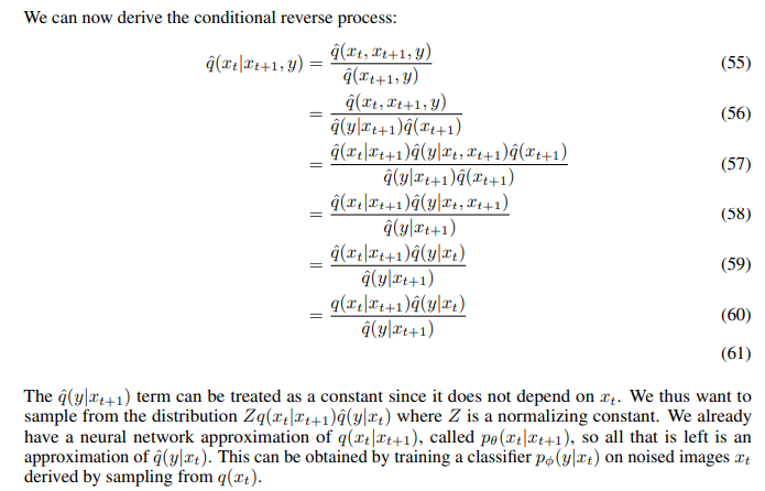
We start with a diffusion model with an unconditional reverse noising process pθ(xt|xt+1). To condition this on a label y, it suffices to sample each transition2 according to

where Z is a normalizing constant (proof in Appendix H). It is typically intractable to sample from this distribution exactly, but Sohl-Dickstein et al. [56] show that it can be approximated as a perturbed Gaussian distribution. Here, we review this derivation.
Recall that our diffusion model predicts the previous timestep xt from timestep xt+1 using a Gaussian distribution:

We can assume that logφ p(y|xt) has low curvature compared to Σ^−1 . This assumption is reasonable in the limit of infinite diffusion steps, where ||Σ|| → 0. In this case, we can approximate log pφ(y|xt) using a Taylor expansion around xt = µ as
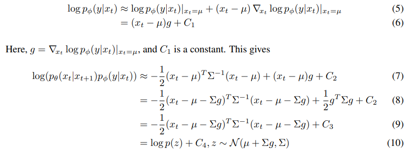
We can safely ignore the constant term C4, since it corresponds to the normalizing coefficient Z in Equation 2. We have thus found that the conditional transition operator can be approximated by a Gaussian similar to the unconditional transition operator, but with its mean shifted by Σg. Algorithm 1 summaries the corresponding sampling algorithm. We include an optional scale factor s for the gradients, which we describe in more detail in Section 4.3.

4.2. Conditional Sampling for DDIM
The above derivation for conditional sampling is only valid for the stochastic diffusion sampling process, and cannot be applied to deterministic sampling methods like DDIM [57]. To this end, we use a score-based conditioning trick adapted from Song et al. [60], which leverages the connection between diffusion models and score matching [59]. In particular, if we have a model ε θ(xt) that predicts the noise added to a sample, then this can be used to derive a score function:

We can now substitute this into the score function for p(xt)p(y|xt):

Finally, we can define a new epsilon prediction εˆ(xt) which corresponds to the score of the joint distribution:

We can then use the exact same sampling procedure as used for regular DDIM, but with the modified noise predictions εˆθ(xt) instead of εθ(xt). Algorithm 2 summaries the corresponding sampling algorithm.
4.3. Scaling Classifier Gradients
To apply classifier guidance to a large scale generative task, we train classification models on ImageNet. Our classifier architecture is simply the downsampling trunk of the UNet model with an attention pool [49] at the 8x8 layer to produce the final output. We train these classifiers on the same noising distribution as the corresponding diffusion model, and also add random crops to reduce overfitting. After training, we incorporate the classifier into the sampling process of the diffusion model using Equation 10, as outlined by Algorithm 1.
In initial experiments with unconditional ImageNet models, we found it necessary to scale the classifier gradients by a constant factor larger than 1. When using a scale of 1, we observed that the classifier assigned reasonable probabilities (around 50%) to the desired classes for the final samples, but these samples did not match the intended classes upon visual inspection. Scaling up the classifier gradients remedied this problem, and the class probabilities from the classifier increased to nearly 100%. Figure 3 shows an example of this effect.
To understand the effect of scaling classifier gradients, note that s · ∇x log p(y|x) = ∇x log 1/Z p(y|x)^s , where Z is an arbitrary constant. As a result, the conditioning process is still theoretically grounded in a re-normalized classifier distribution proportional to p(y|x)^s . When s > 1, this distribution becomes sharper than p(y|x), since larger values are amplified by the exponent. In other words, using a larger gradient scale focuses more on the modes of the classifier, which is potentially desirable for producing higher fidelity (but less diverse) samples.
In the above derivations, we assumed that the underlying diffusion model was unconditional, modeling p(x). It is also possible to train conditional diffusion models, p(x|y), and use classifier guidance in the exact same way. Table 4 shows that the sample quality of both unconditional and conditional models can be greatly improved by classifier guidance. We see that, with a high enough scale, the guided unconditional model can get quite close to the FID of an unguided conditional model, although training directly with the class labels still helps. Guiding a conditional model further improves FID.
Table 4 also shows that classifier guidance improves precision at the cost of recall, thus introducing a trade-off in sample fidelity versus diversity. We explicitly evaluate how this trade-off varies with the gradient scale in Figure 4. We see that scaling the gradients beyond 1.0 smoothly trades off recall (a measure of diversity) for higher precision and IS (measures of fidelity). Since FID and sFID depend on both diversity and fidelity, their best values are obtained at an intermediate point. We also compare our guidance with the truncation trick from BigGAN in Figure 5. We find that classifier guidance is strictly better than BigGAN-deep when trading off FID for Inception Score. Less clear cut is the precision/recall trade-off, which shows that classifier guidance is only a better choice up until a certain precision threshold, after which point it cannot achieve better precision.


5. Results
To evaluate our improved model architecture on unconditional image generation, we train separate diffusion models on three LSUN [71] classes: bedroom, horse, and cat. To evaluate classifier guidance, we train conditional diffusion models on the ImageNet [52] dataset at 128×128, 256×256, and 512×512 resolution.
5.1. State-of-the-art Image Synthesis
Table 5 summarizes our results. Our diffusion models can obtain the best FID on each task, and the best sFID on all but one task. With the improved architecture, we already obtain state-of-the-art image generation on LSUN and ImageNet 64×64. For higher resolution ImageNet, we observe that classifier guidance allows our models to substantially outperform the best GANs. These models obtain perceptual quality similar to GANs, while maintaining a higher coverage of the distribution as measured by recall, and can even do so using only 25 diffusion steps.
Figure 6 compares random samples from the best BigGAN-deep model to our best diffusion model. While the samples are of similar perceptual quality, the diffusion model contains more modes than the GAN, such as zoomed ostrich heads, single flamingos, different orientations of cheeseburgers, and a tinca fish with no human holding it. We also check our generated samples for nearest neighbors in the Inception-V3 feature space in Appendix C, and we show additional samples in Appendices K-M.


5.2. Comparison to Upsampling
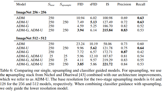
We also compare guidance to using a two-stage upsampling stack. Nichol and Dhariwal [43] and Saharia et al. [53] train two-stage diffusion models by combining a low-resolution diffusion model with a corresponding upsampling diffusion model. In this approach, the upsampling model is trained to upsample images from the training set, and conditions on low-resolution images that are concatenated channel-wise to the model input using a simple interpolation (e.g. bilinear). During sampling, the low-resolution model produces a sample, and then the upsampling model is conditioned on this sample. This greatly improves FID on ImageNet 256×256, but does not reach the same performance as state-of-the-art models like BigGAN-deep [43, 53], as seen in Table 5.
In Table 6, we show that guidance and upsampling improve sample quality along different axes. While upsampling improves precision while keeping a high recall, guidance provides a knob to trade off diversity for much higher precision. We achieve the best FIDs by using guidance at a lower resolution before upsampling to a higher resolution, indicating that these approaches complement one another.
6. Related Work
Score based generative models were introduced by Song and Ermon [59] as a way of modeling a data distribution using its gradients, and then sampling using Langevin dynamics [67]. Ho et al. [25] found a connection between this method and diffusion models [56], and achieved excellent sample quality by leveraging this connection. After this breakthrough work, many works followed up with more promising results: Kong et al. [30] and Chen et al. [8] demonstrated that diffusion models work well for audio; Jolicoeur-Martineau et al. [26] found that a GAN-like setup could improve samples from these models; Song et al. [60] explored ways to leverage techniques from stochastic differential equations to improve the sample quality obtained by score-based models; Song et al. [57] and Nichol and Dhariwal [43] proposed methods to improve sampling speed; Nichol and Dhariwal [43] and Saharia et al. [53] demonstrated promising results on the difficult ImageNet generation task using upsampling diffusion models. Also related to diffusion models, and following the work of Sohl-Dickstein et al. [56], Goyal et al. [21] described a technique for learning a model with learned iterative generation steps, and found that it could achieve good image samples when trained with a likelihood objective.
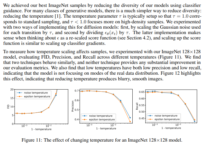
One missing element from previous work on diffusion models is a way to trade off diversity for fidelity. Other generative techniques provide natural levers for this trade-off. Brock et al. [5] introduced the truncation trick for GANs, wherein the latent vector is sampled from a truncated normal distribution. They found that increasing truncation naturally led to a decrease in diversity but an increase in fidelity. More recently, Razavi et al. [51] proposed to use classifier rejection sampling to filter out bad samples from an autoregressive likelihood-based model, and found that this technique improved FID. Most likelihood-based models also allow for low-temperature sampling [1], which provides a natural way to emphasize modes of the data distribution (see Appendix G).
Other likelihood-based models have been shown to produce high-fidelity image samples. VQ-VAE [65] and VQ-VAE-2 [51] are autoregressive models trained on top of quantized latent codes, greatly reducing the computational resources required to train these models on large images. These models produce diverse and high quality images, but still fall short of GANs without expensive rejection sampling and special metrics to compensate for blurriness. DCTransformer [42] is a related method which relies on a more intelligent compression scheme. VAEs are another promising class of likelihood-based models, and recent methods such as NVAE [63] and VDVAE [9] have successfully been applied to difficult image generation domains. Energy-based models are another class of likelihood-based models with a rich history [1, 10, 24]. Sampling from the EBM distribution is challenging, and Xie et al. [70] demonstrate that Langevin dynamics can be used to sample coherent images from these models. Du and Mordatch [15] further improve upon this approach, obtaining high quality images. More recently, Gao et al. [18] incorporate diffusion steps into an energy-based model, and find that doing so improves image samples from these models.
Other works have controlled generative models with a pre-trained classifier. For example, an emerging body of work [17, 47, 2] aims to optimize GAN latent spaces for text prompts using pre-trained CLIP [49] models. More similar to our work, Song et al. [60] uses a classifier to generate class-conditional CIFAR-10 images with a diffusion model. In some cases, classifiers can act as stand-alone generative models. For example, Santurkar et al. [55] demonstrate that a robust image classifier can be used as a stand-alone generative model, and Grathwohl et al. [22] train a model which is jointly a classifier and an energy-based model.
7. Limitations and Future Work
While we believe diffusion models are an extremely promising direction for generative modeling, they are still slower than GANs at sampling time due to the use of multiple denoising steps (and therefore forward passes). One promising work in this direction is from Luhman and Luhman [37], who explore a way to distill the DDIM sampling process into a single step model. The samples from the single step model are not yet competitive with GANs, but are much better than previous single-step likelihood-based models. Future work in this direction might be able to completely close the sampling speed gap between diffusion models and GANs without sacrificing image quality.
Our proposed classifier guidance technique is currently limited to labeled datasets, and we have provided no effective strategy for trading off diversity for fidelity on unlabeled datasets. In the future, our method could be extended to unlabeled data by clustering samples to produce synthetic labels [36] or by training discriminative models to predict when samples are in the true data distribution or from the sampling distribution.
The effectiveness of classifier guidance demonstrates that we can obtain powerful generative models from the gradients of a classification function. This could be used to condition pre-trained models in a plethora of ways, for example by conditioning an image generator with a text caption using a noisy version of CLIP [49], similar to recent methods that guide GANs using text prompts [17, 47, 2]. It also suggests that large unlabeled datasets could be leveraged in the future to pre-train powerful diffusion models that can later be improved by using a classifier with desirable properties.
8. Conclusion
We have shown that diffusion models, a class of likelihood-based models with a stationary training objective, can obtain better sample quality than state-of-the-art GANs. Our improved architecture is sufficient to achieve this on unconditional image generation tasks, and our classifier guidance technique allows us to do so on class-conditional tasks. In the latter case, we find that the scale of the classifier gradients can be adjusted to trade off diversity for fidelity. These guided diffusion models can reduce the sampling time gap between GANs and diffusion models, although diffusion models still require multiple forward passes during sampling. Finally, by combining guidance with upsampling, we can further improve sample quality on high-resolution conditional image synthesis.
A. Computational Requirements
Compute is essential to modern machine learning applications, and more compute typically yields better results. It is thus important to compare our method’s compute requirements to competing methods. In this section, we demonstrate that we can achieve results better than StyleGAN2 and BigGAN-deep with the same or lower compute budget.
A.1. Throughput
We first benchmark the throughput of our models in Table 7. For the theoretical throughput, we measure the theoretical FLOPs for our model using THOP [73], and assume 100% utilization of an NVIDIA Tesla V100 (120 TFLOPs), while for the actual throughput we use measured wall-clock time. We include communication time across two machines whenever our training batch size doesn’t fit on a single machine, where each of our machines has 8 V100s.
We find that a naive implementation of our models in PyTorch 1.7 is very inefficient, utilizing only 20-30% of the hardware. We also benchmark our optimized version, which use larger per-GPU batch sizes, fused GroupNorm-Swish and fused Adam CUDA ops. For our ImageNet 128×128 model in particular, we find that we can increase the per-GPU batch size from 4 to 32 while still fitting in GPU memory, and this makes a large utilization difference. Our implementation is still far from optimal, and further optimizations should allow us to reach higher levels of utilization.

A.2. Early stopping
In addition, we can train for many fewer iterations while maintaining sample quality superior to BigGAN-deep. Table 8 and 9 evaluate our ImageNet 128×128 and 256×256 models throughout training. We can see that the ImageNet 128×128 model beats BigGAN-deep’s FID (6.02) after 500K training iterations, only one eighth of the way through training. Similarly, the ImageNet 256×256 model beats BigGAN-deep after 750K iterations, roughly a third of the way through training.


A.3. Compute comparison
Finally, in Table 10 we compare the compute of our models with StyleGAN2 and BigGAN-deep, and show we can obtain better FIDs with a similar compute budget. For BigGAN-deep, Brock et al. [5] do not explicitly describe the compute requirements for training their models, but rather provide rough estimates in terms of days on a Google TPUv3 pod [20]. We convert their TPU-v3 estimates to V100 days according to 2 TPU-v3 day = 1 V100 day. For StyleGAN2, we use the reported throughput of 25M images over 32 days 13 hour on one V100 for config-f [44]. We note that our classifier training is relatively lightweight compared to training the generative model.

B. Detailed Formulation of DDPM


C. Nearest Neighbors for Samples

Our models achieve their best FID when using a classifier to reduce the diversity of the generations. One might fear that such a process could cause the model to recall existing images from the training dataset, especially as the classifier scale is increased. To test this, we looked at the nearest neighbors (in InceptionV3 [62] feature space) for a handful of samples. Figure 7 shows our results, revealing that the samples are indeed unique and not stored in the training set.
D. Effect of Varying the Classifier Scale

E. LSUN Diversity Comparison

G. Reduced Temperature Sampling

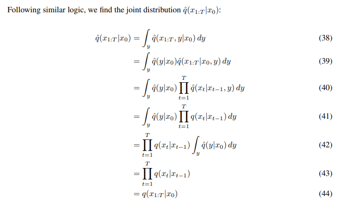
H. Conditional Diffusion Process


'*Generative Model > Diffusion' 카테고리의 다른 글
Progressive Distillation for Fast Sampling of Diffusion Models (0) 2025.01.23 Denoising Diffusion Implicit Models (0) 2025.01.23 High-Resolution Image Synthesis with Latent Diffusion Models (0) 2024.08.23 Improved Denoising Diffusion Probabilistic Models (0) 2024.08.20