Denoising Diffusion Implicit Models

https://arxiv.org/pdf/2010.02502

(Oct 2022 ICLR 2021)

https://github.com/ermongroup/ddim

---

---

Abstract

Denoising diffusion probabilistic models (DDPMs) have achieved high quality image generation without adversarial training, yet they require simulating a Markov chain for many steps in order to produce a sample. To accelerate sampling, we present denoising diffusion implicit models (DDIMs), a more efficient class of iterative implicit probabilistic models with the same training procedure as DDPMs. In DDPMs, the generative process is defined as the reverse of a particular Markovian diffusion process. We generalize DDPMs via a class of non-Markovian diffusion processes that lead to the same training objective. These non-Markovian processes can correspond to generative processes that are deterministic, giving rise to implicit models that produce high quality samples much faster. We empirically demonstrate that DDIMs can produce high quality samples 10× to 50× faster in terms of wall-clock time compared to DDPMs, allow us to trade off computation for sample quality, perform semantically meaningful image interpolation directly in the latent space, and reconstruct observations with very low error.

---

1. Introduction

Deep generative models have demonstrated the ability to produce high quality samples in many domains (Karras et al., 2020; van den Oord et al., 2016a). In terms of image generation, generative adversarial networks (GANs, Goodfellow et al. (2014)) currently exhibits higher sample quality than likelihood-based methods such as variational autoencoders (Kingma & Welling, 2013), autoregressive models (van den Oord et al., 2016b) and normalizing flows (Rezende & Mohamed, 2015; Dinh et al., 2016). However, GANs require very specific choices in optimization and architectures in order to stabilize training (Arjovsky et al., 2017; Gulrajani et al., 2017; Karras et al., 2018; Brock et al., 2018), and could fail to cover modes of the data distribution (Zhao et al., 2018).

 

Recent works on iterative generative models (Bengio et al., 2014), such as denoising diffusion probabilistic models (DDPM, Ho et al. (2020)) and noise conditional score networks (NCSN, Song & Ermon (2019)) have demonstrated the ability to produce samples comparable to that of GANs, without having to perform adversarial training. To achieve this, many denoising autoencoding models are trained to denoise samples corrupted by various levels of Gaussian noise. Samples are then produced by a Markov chain which, starting from white noise, progressively denoises it into an image. This generative Markov Chain process is either based on Langevin dynamics (Song & Ermon, 2019) or obtained by reversing a forward diffusion process that progressively turns an image into noise (Sohl-Dickstein et al., 2015).

 

A critical drawback of these models is that they require many iterations to produce a high quality sample. For DDPMs, this is because that the generative process (from noise to data) approximates the reverse of the forward diffusion process (from data to noise), which could have thousands of steps; iterating over all the steps is required to produce a single sample, which is much slower compared to GANs, which only needs one pass through a network. For example, it takes around 20 hours to sample 50k images of size 32 × 32 from a DDPM, but less than a minute to do so from a GAN on a Nvidia 2080 Ti GPU. This becomes more problematic for larger images as sampling 50k images of size 256 × 256 could take nearly 1000 hours on the same GPU.

 

To close this efficiency gap between DDPMs and GANs, we present denoising diffusion implicit models (DDIMs). DDIMs are implicit probabilistic models (Mohamed & Lakshminarayanan, 2016) and are closely related to DDPMs, in the sense that they are trained with the same objective function.

 

In Section 3, we generalize the forward diffusion process used by DDPMs, which is Markovian, to non-Markovian ones, for which we are still able to design suitable reverse generative Markov chains. We show that the resulting variational training objectives have a shared surrogate objective, which is exactly the objective used to train DDPM. Therefore, we can freely choose from a large family of generative models using the same neural network simply by choosing a different, non-Markovian diffusion process (Section 4.1) and the corresponding reverse generative Markov Chain. In particular, we are able to use non-Markovian diffusion processes which lead to ”short” generative Markov chains (Section 4.2) that can be simulated in a small number of steps. This can massively increase sample efficiency only at a minor cost in sample quality.

 

In Section 5, we demonstrate several empirical benefits of DDIMs over DDPMs. First, DDIMs have superior sample generation quality compared to DDPMs, when we accelerate sampling by 10× to 100× using our proposed method. Second, DDIM samples have the following “consistency” property, which does not hold for DDPMs: if we start with the same initial latent variable and generate several samples with Markov chains of various lengths, these samples would have similar high-level features. Third, because of “consistency” in DDIMs, we can perform semantically meaningful image interpolation by manipulating the initial latent variable in DDIMs, unlike DDPMs which interpolates near the image space due to the stochastic generative process.

---

2. Background

---

3. Variational Inference for Non-Markovian Forward Processes

---

3.1. Non-Markovian Forward Processes

 

---

3.2. Generative Process and Unified Variational Inference Objective

---

4. Sampling from Generailized Generative Processes

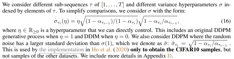
With L1 as the objective, we are not only learning a generative process for the Markovian inference process considered in Sohl-Dickstein et al. (2015) and Ho et al. (2020), but also generative processes for many non-Markovian forward processes parametrized by σ that we have described. Therefore, we can essentially use pretrained DDPM models as the solutions to the new objectives, and focus on finding a generative process that is better at producing samples subject to our needs by changing σ.

---

4.1. Denoising Diffusion Implicit Models

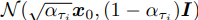
where εt ∼ N (0, I) is standard Gaussian noise independent of xt, and we define α0 := 1. Different choices of σ values results in different generative processes, all while using the same model εθ, so re-training the model is unnecessary.

 

When

 

the forward process becomes Markovian, and the generative process becomes a DDPM.

 

We note another special case when σt = 0 for all t 5 ; the forward process becomes deterministic given xt−1 and x0, except for t = 1; in the generative process, the coefficient before the random noise εt becomes zero. The resulting model becomes an implicit probabilistic model (Mohamed & Lakshminarayanan, 2016), where samples are generated from latent variables with a fixed procedure (from xT to x0). We name this the denoising diffusion implicit model (DDIM, pronounced /d:Im/), because it is an implicit probabilistic model trained with the DDPM objective (despite the forward process no longer being a diffusion).

---

4.2. Accelerated Generation Processes

In the previous sections, the generative process is considered as the approximation to the reverse process; since of the forward process has T steps, the generative process is also forced to sample T steps. However, as the denoising objective L1 does not depend on the specific forward procedure as long as qσ(xt|x0) is fixed, we may also consider forward processes with lengths smaller than T, which accelerates the corresponding generative processes without having to train a different model.

 

Let us consider the forward process as defined not on all the latent variables x1:T, but on a subset {xτ1 , . . . , xτS }, where τ is an increasing sub-sequence of [1, . . . , T] of length S. In particular, we define the sequential forward process over x_τ1 , . . . , x_τS such that q(xτi |x0) =

 

matches the “marginals” (see Figure 2 for an illustration).

 

The generative process now samples latent variables according to reversed(τ), which we term (sampling) trajectory. When the length of the sampling trajectory is much smaller than T, we may achieve significant increases in computational efficiency due to the iterative nature of the sampling process.

 

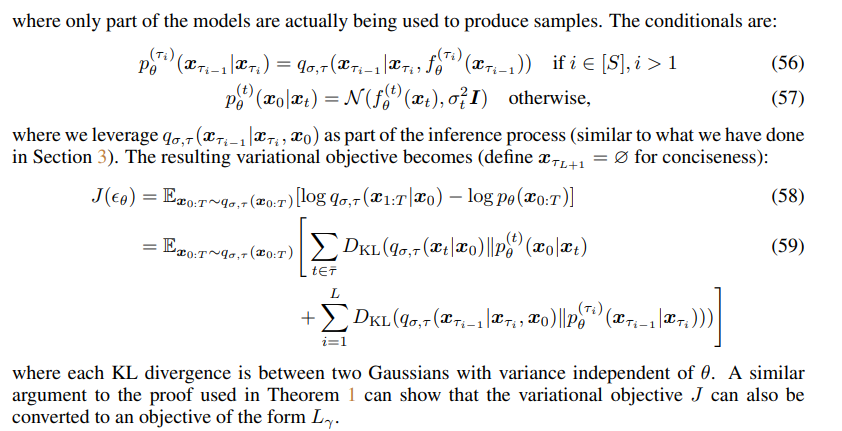
Using a similar argument as in Section 3, we can justify using the model trained with the L1 objective, so no changes are needed in training. We show that only slight changes to the updates in Eq. (12) are needed to obtain the new, faster generative processes, which applies to DDPM, DDIM, as well as all generative processes considered in Eq. (10). We include these details in Appendix C.1.

 

In principle, this means that we can train a model with an arbitrary number of forward steps but only sample from some of them in the generative process. Therefore, the trained model could consider many more steps than what is considered in (Ho et al., 2020) or even a continuous time variable t (Chen et al., 2020). We leave empirical investigations of this aspect as future work.

---

4.3. Relevance to Neural ODEs

---

5. Experiments

In this section, we show that DDIMs outperform DDPMs in terms of image generation when fewer iterations are considered, giving speed ups of 10× to 100× over the original DDPM generation process. Moreover, unlike DDPMs, once the initial latent variables xT are fixed, DDIMs retain high-level image features regardless of the generation trajectory, so they are able to perform interpolation directly from the latent space. DDIMs can also be used to encode samples that reconstruct them from the latent code, which DDPMs cannot do due to the stochastic sampling process.

 

For each dataset, we use the same trained model with T = 1000 and the objective being Lγ from Eq. (5) with γ = 1; as we argued in Section 3, no changes are needed with regards to the training procedure. The only changes that we make is how we produce samples from the model; we achieve this by controlling τ (which controls how fast the samples are obtained) and σ (which interpolates between the deterministic DDIM and the stochastic DDPM).

---

5.1. Sample Quality and Efficiency

In Table 1, we report the quality of the generated samples with models trained on CIFAR10 and CelebA, as measured by Frechet Inception Distance (FID (Heusel et al., 2017)), where we vary the number of timesteps used to generate a sample (dim(τ )) and the stochasticity of the process (η). As expected, the sample quality becomes higher as we increase dim(τ ), presenting a tradeoff between sample quality and computational costs. We observe that DDIM (η = 0) achieves the best sample quality when dim(τ ) is small, and DDPM (η = 1 and σˆ) typically has worse sample quality compared to its less stochastic counterparts with the same dim(τ ), except for the case for dim(τ ) = 1000 and σˆ reported by Ho et al. (2020) where DDIM is marginally worse. However, the sample quality of σˆ becomes much worse for smaller dim(τ ), which suggests that it is ill-suited for shorter trajectories. DDIM, on the other hand, achieves high sample quality much more consistently.

 

In Figure 3, we show CIFAR10 and CelebA samples with the same number of sampling steps and varying σ. For the DDPM, the sample quality deteriorates rapidly when the sampling trajectory has 10 steps. For the case of σˆ, the generated images seem to have more noisy perturbations under short trajectories; this explains why the FID scores are much worse than other methods, as FID is very sensitive to such perturbations (as discussed in Jolicoeur-Martineau et al. (2020)).

 

In Figure 4, we show that the amount of time needed to produce a sample scales linearly with the length of the sample trajectory. This suggests that DDIM is useful for producing samples more efficiently, as samples can be generated in much fewer steps. Notably, DDIM is able to produce samples with quality comparable to 1000 step models within 20 to 100 steps, which is a 10× to 50× speed up compared to the original DDPM. Even though DDPM could also achieve reasonable sample quality with 100× steps, DDIM requires much fewer steps to achieve this; on CelebA, the FID score of the 100 step DDPM is similar to that of the 20 step DDIM.

---

5.2. Sample Consistency in DDIMs

For DDIM, the generative process is deterministic, and x0 would depend only on the initial state xT . In Figure 5, we observe the generated images under different generative trajectories (i.e. different τ ) while starting with the same initial xT . Interestingly, for the generated images with the same initial xT , most high-level features are similar, regardless of the generative trajectory. In many cases, samples generated with only 20 steps are already very similar to ones generated with 1000 steps in terms of high-level features, with only minor differences in details. Therefore, it would appear that xT alone would be an informative latent encoding of the image; and minor details that affects sample quality are encoded in the parameters, as longer sample trajectories gives better quality samples but do not significantly affect the high-level features. We show more samples in Appendix D.4.

---

5.3. Interpolation in Deterministic Generative Processes

Since the high level features of the DDIM sample is encoded by xT , we are interested to see whether it would exhibit the semantic interpolation effect similar to that observed in other implicit probabilistic models, such as GANs (Goodfellow et al., 2014). This is different from the interpolation procedure in Ho et al. (2020), since in DDPM the same xT would lead to highly diverse x0 due to the stochastic generative process6 . In Figure 6, we show that simple interpolations in xT can lead to semantically meaningful interpolations between two samples. We include more details and samples in Appendix D.5. This allows DDIM to control the generated images on a high level directly through the latent variables, which DDPMs cannot.

---

5.4. Reconstruction from Latent Space

As DDIM is the Euler integration for a particular ODE, it would be interesting to see whether it can encode from x0 to xT (reverse of Eq. (14)) and reconstruct x0 from the resulting xT (forward of Eq. (14))7 . We consider encoding and decoding on the CIFAR-10 test set with the CIFAR-10 model with S steps for both encoding and decoding; we report the per-dimension mean squared error (scaled to [0, 1]) in Table 2. Our results show that DDIMs have lower reconstruction error for larger S values and have properties similar to Neural ODEs and normalizing flows. The same cannot be said for DDPMs due to their stochastic nature.

---

6. Related Work

Our work is based on a large family of existing methods on learning generative models as transition operators of Markov chains (Sohl-Dickstein et al., 2015; Bengio et al., 2014; Salimans et al., 2014; Song et al., 2017; Goyal et al., 2017; Levy et al., 2017). Among them, denoising diffusion probabilistic models (DDPMs, Ho et al. (2020)) and noise conditional score networks (NCSN, Song & Ermon (2019; 2020)) have recently achieved high sample quality comparable to GANs (Brock et al., 2018; Karras et al., 2018). DDPMs optimize a variational lower bound to the log-likelihood, whereas NCSNs optimize the score matching objective (Hyvarinen ¨ , 2005) over a nonparametric Parzen density estimator of the data (Vincent, 2011; Raphan & Simoncelli, 2011).

 

Despite their different motivations, DDPMs and NCSNs are closely related. Both use a denoising autoencoder objective for many noise levels, and both use a procedure similar to Langevin dynamics to produce samples (Neal et al., 2011). Since Langevin dynamics is a discretization of a gradient flow (Jordan et al., 1998), both DDPM and NCSN require many steps to achieve good sample quality. This aligns with the observation that DDPM and existing NCSN methods have trouble generating high-quality samples in a few iterations.

 

DDIM, on the other hand, is an implicit generative model (Mohamed & Lakshminarayanan, 2016) where samples are uniquely determined from the latent variables. Hence, DDIM has certain properties that resemble GANs (Goodfellow et al., 2014) and invertible flows (Dinh et al., 2016), such as the ability to produce semantically meaningful interpolations. We derive DDIM from a purely variational perspective, where the restrictions of Langevin dynamics are not relevant; this could partially explain why we are able to observe superior sample quality compared to DDPM under fewer iterations. The sampling procedure of DDIM is also reminiscent of neural networks with continuous depth (Chen et al., 2018; Grathwohl et al., 2018), since the samples it produces from the same latent variable have similar high-level visual features, regardless of the specific sample trajectory.

---

7. Discussion

We have presented DDIMs – an implicit generative model trained with denoising auto-encoding / score matching objectives – from a purely variational perspective. DDIM is able to generate high quality samples much more efficiently than existing DDPMs and NCSNs, with the ability to perform meaningful interpolations from the latent space. The non-Markovian forward process presented here seems to suggest continuous forward processes other than Gaussian (which cannot be done in the original diffusion framework, since Gaussian is the only stable distribution with finite variance). We also demonstrated a discrete case with a multinomial forward process in Appendix A, and it would be interesting to investigate similar alternatives for other combinatorial structures.

 

Moreover, since the sampling procedure of DDIMs is similar to that of an neural ODE, it would be interesting to see if methods that decrease the discretization error in ODEs, including multistep methods such as Adams-Bashforth (Butcher & Goodwin, 2008), could be helpful for further improving sample quality in fewer steps (Queiruga et al., 2020). It is also relevant to investigate whether DDIMs exhibit other properties of existing implicit models (Bau et al., 2019).

---

---

---