8. Unobserved Confounding: Bounds and Sensitivity Analysis

https://www.bradyneal.com/causal-inference-course#course-textbook

---

All of the methods in Chapter 7 assume that we don't have any unobserved confounding. However, unconfoundedness is an untestable assumption. In observational studies, there could also be some unobserved confounder(s). Therefore, we'd like to know how robust our estimates are to unobserved confounding.

 

The first way we can do is by getting an upper and lower bound on the causal effect using credible assumptions.

 

Another way we can do this is by simulating how strong the confounder's effect on the treatment and the counfounder's effect on the outcome need to be to make the true causal effect substantially different from our estimate.

---

8.1. Bounds

There is a tradeoff between how realistic or credible our assumptions are and how precise of an identification result we can get. Manski calls this "The Law of Decreasing Credibility: the credibility of inference dereases with the strength of the assumptions maintained."

 

Depending on what assumptions we are willing to make, we can derive various nonparametric bounds on causal effects. We have seen that if we are willing to assume unconfoundedness (or some causal graph in which the causal effect is identifiable) and positivity, we can identify a single point for the causal effect. However, this might be unrealistic. For example, there could always be unobserved confounding in observational studies.

 

This is what motivates Charles Manski's work on bounding causal effects. This gives us an interval that the causal effect must be in, rather than telling us exactly what point in that interval the causal effect must be. In this section, we will give an introduction to these nonparametric bounds and how to derive them.

 

The assumptions that we consider are weaker than unconfoundedness, so they give us intervals that the causal effect must fall in (under these assumptions). If we assumed the stronger assumption of unconfoundedness, these intervals would collapse to a single point. This illustrates the law of decreasing credibility.

---

8.1.1. No-Assumptions Bound

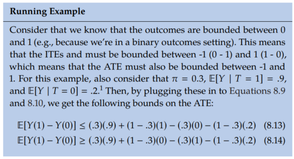
Say all we know about the potential outcomes Y(0) and Y(1) is that they are between 0 and 1. Then, the maximum value of an ITE Yi(1) - Yi(0) is 1 (1-0), and the minimum is -1 (0-1):

 

So we know that all ITEs must be in an interval of length 2. Because all the ITEs must fall inside this interval of length 2, the ATE must also fall inside this interval of length 2.

 

Interestingly, for ATEs, it turns out that we can cut the length of this interval in half without making any assumptions (beyond the min/max value of outcome); the interval that the ATE must fall in is only of length 1.

 

We'll show this result from Manski in the more general scenario where the outcome is bounded between a and b:

 

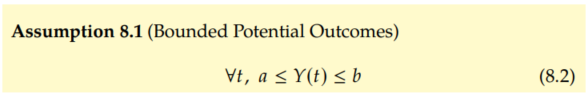
By the same reasoning as above, this implies the following bounds on the ITEs and ATE:

 

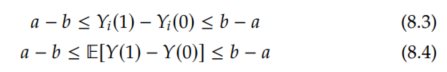
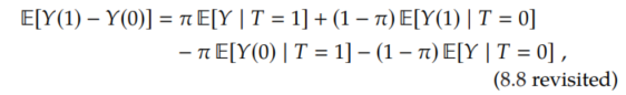
These are intervals of length (b-a)-(a-b) = 2(b-a). And the bounds for the ITEs cannot be made tighter without further assumptions. However, seemingly magically, we can halve the length of the interval for the ATE. To see this, we rewrite the ATE as follows:

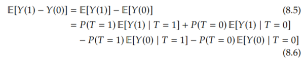
We immediately recognize the first and last terms as friendly conditional expectations that we can estimate from observational data:

 

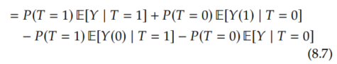
Because this is such an important decomposition, we'll give it a name and box before moving on with the bound derivation. We will call this the observational-counterfactual decomposition (of the ATE). Also, to have a bit more concise notation, we'll use

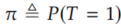
moving forward.

 

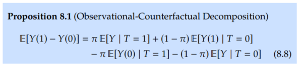
Unfortunately, E[Y(1) | T=0] and E[Y(0) | T=1] are counterfactual. However, we know that they're bounded between a and b. Therefore, we get an upper bound on the complete expression by letting the quantity that's being added (E[Y(1) | T=0]) equal b and letting the quantity that's being subtracted (E[Y(0) | T=1]) equal a. Similarly, we can get a lower bound by letting the term that's being added equal a and the term that's being subtracted equal b.

 

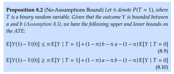
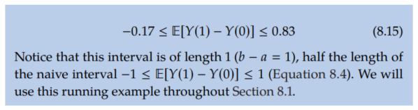
Importantly, the length of this interval is b - a, half the length of the naive interval that we saw in Equation 8.4. We can see this by subtracting the lower bound from the upper bound:

 

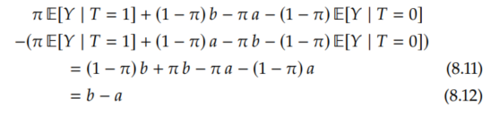
This is sometimes referred to as the "no-assumptions bound" because we made no assumptions other than that the outcomes are bounded. If the outcomes are not bounded, then the ATE and ITEs can be anywhere between -∞ and ∞.

 

The bounds in Proposition 8.2 are as tight as we can get without further assumptions. Unfortunately, the corresponding interval always contains 0, which means that we cannot use this bound to distinguish "no causal effect" from "causal effect." Can we get tighter bounds?

 

(To see the no-assumptions bound always contains zero, consider what we would need for it to not contain zero: we would either need the upper bound to be less than zero or the lower bound to be greater than zero. However, this cannot be the case. To see why, note that the minimum upper bound is achieved when E[Y | T=1] = a and E[Y | T=0] = b, which gives us an (inclusive) upper bound of zero. Same with the lower bound. (maximum lower bound is 0.))

 

In order to bound the ATE, we must have some information about the counterfactual part of this decomposition. We can easily estimate the observational part from data. In the no-assumptions bound (Proposition 8.2), all we assumed is that the outcomes are bounded by a and b. 

 

If we make more assumptions, we can get smaller intervals. In the next few sections, we will cover some assumptions that are sometimes fairly reasonable, depending on the setting, and what tighter bounds these assumptions get us. The general strategy we will use for all of them is to start with the observational-counterfactual decomposition of the ATE (Proposition 8.1),

 

and get smaller intervals by bounding the counterfactual parts using the different assumptions we make.

 

The intervals we will see in the next couple of subsections will all contain zero. We won't see an interval that is purely positive or purely negative until Section 8.1.4.

---

8.1.2. Monotone Treatment Response

For our first assumption beyond assuming bounded outcomes, consider that we find ourselves in a setting where it is feasible that the treatment can only help; it can't hurt. This is the setting that Manski considers in context. In this setting, we can justify the monotone treatment response (MTR) assumption:

 

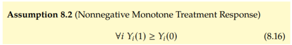
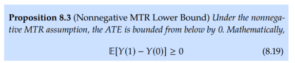
This means that every ITE is nonnegative, so we can bring our lower ound on the ITEs up from a - b (Equation 8.3) to 0. So, intuitively, this should mean that our lower bound on the ATE should move up to 0. And we will now see that this is the case.

 

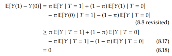
Now, rather than lower bounding E[Y(1) | T=0] with a and -E[Y(0) | T=1] with -b, we can do better. Because the treatment only helps, E[Y(1) | T=0] ≥ E[Y(0) | T=0] = E[Y | T=0], so we can lower bound E[Y(1) | T=0] with E[Y | T=0]. Similarly, -E[Y(0) | T=1] ≥ -E[Y(1) | T=1] = -E[Y | T=1] (since multiplying by a negative flips the inequality), so we can lower bound -E[Y(0) | T=1] with -E[Y | T=1]. 

 

Therefore, we can improve on the no-assumptions lower bound to get 0, as our intuition suggested:

Running Example

The no-assumptions upper bound still applies here, so in our running example from Section 8.1.1 where π=.3, E[Y | T=1] = .9, and E[Y | T=0] = .2, our ATE interval improves from [-0.17, 0.83] (Equation 8.15) to [0, 0.83].

 

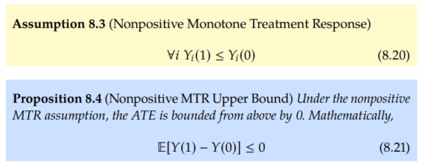
Alternatively, say the treatment can only hurt people; it can't help them (e.g. a gunshot would only hurts chances of staying alive ㅜㅜ 이렇게 무서운 비유라니..). In those cases, we would have the nonpositive monotone treatment response assumption and the nonpositive MTR upper bound:

Running Example

And in this setting, the no-assumptions lower bound wtill applies. That means that the ATE interval in our example improves from [-0.17,0.83] (Equation 8.15) to [-0.17, 0].

---

8.1.3. Monotone Treatment Selection

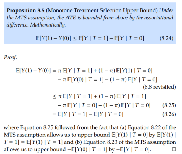
The next assumption that we'll consider is the assumption that the people who selected treatment would have better outcomes than those who didn't select treatment, under either treatment scenario. Manski and Pepper introduced this as the monotone treatment selection (MTS) assumption.

 

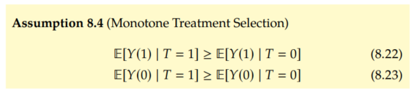
As Morgan and Winship point out, you might think of this as positive self-selection. Those who generally get better outcomes self-select into the treatment group. 

 

Again, we start with the observational-counterfactual decomposition, and we now obtain an upper bound using the MTS assumption (Assumption 8.4):

Running Example

Recall our running example from Section 8.1.1. where π=.3, E[Y | T=1] = .9, E[Y | T=0] = .2. The MTS assumption gives us an upper bound, and we still have the no-assumptions lower bound. That means that the ATE interval in our example improves from [-0.17, 0.83] (Equation 8.15) to [-0.17, 0.7].

Both MTR and MTS

Then, we can combine the nonnegative MTR assumption (Assumption 8.2) with the MTS assumption (Assumption 8.4) to get the lower bound in Proposition 8.3 and the upper bound in Proposition 8.5, respectively. In our running example, this yields the following interval for the ATE: [0, 0.7].

Intervals Contain Zero

Although bounds from the MTR and MTS assumptions can be useful ruling out very large or very small causal effects, the corresponding interval still contain zero. This means that these assumptions are not enough to identify whether there is an effect or not.

---

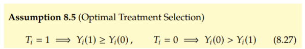
8.1.4. Optimal Treatment Selection

We now consider what we will call the optimal treatment selection (OTS) assumption from Manski. This assumption means that the individuals always receive the treatment that is best for them (e.g. if an expert doctor is deciding which treatment to give people). We write this mathematically as follows:

 

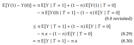
From the OTS assumptions, we know that

 

Therefore, we can give an upper bound, by upper bounding E[Y(1) | T=0] with E[Y | T=0] and upper bounding -E[Y(0) | T=1] with -a (same as in the no-assumptions upper bound):

 

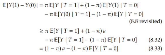
The OTS assumption also tells us that

 

which is equivalent to saying -E[Y(0) | T=1] ≥ -E[Y | T=1]. So we can lower bound -E[Y(0) | T=1] with -E[Y | T=1], and we can lower bound E[Y(1) | T=0] with a (just as we did in the no-assumptions lower bound) to get the following lower bound:

 

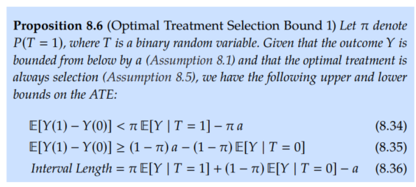
Unfortunately, this interval also always contains zero! This means that Proposition 8.6 doesn't tell us whether the causal effect is non-zero or not.

Running Example 

Recall our running example from Section 8.1.1 where a = 0, b = 1, π = .3, E[Y | T=1] = .9, and E[Y | T=0] = .2. Plugging these in to Proposition 8.6 gives us the following:

 

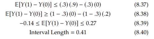
We'll now give an interval that can be purely positive or purely negative, potentially identifying the ATE as non-zero.

A Bound That Can Identify the Sign of the ATE

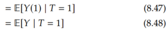
It turns out that, although we take the OTS assumption from Manski, the bound we gave in Proposition 8.6 is not actually the bound that Manski derives with that assumption. For example, where we used E[Y(1) | T=0] ≤ E[Y | T=0], Manski uses E[Y(1) | T=0] ≤ E[Y | T=1]. We'll quickly prove this inequality that Manski uses from the OTS assumption:

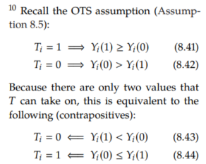
We start by applying Equation 8.42:

 

Because the random variable we are taking the expectation of is Y(1), if we flip Y(0) > Y(1) to Y(0) ≤ Y(1), then we get an upper bound:

 

Finally, applying Equation 8.44, we have the result:

 

Now that we have that E[Y(1) | T=0] ≤ E[Y | T=1], we can prove Manski's upper bound, where we use this key inequality in Equation 8.49:

 

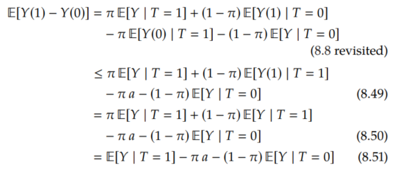
Similarly, we can perform an analogous derivation to get the lower bound:

 

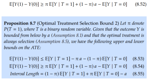
This interval can also include zero, but it doesn't have to. For example, in our running example, it doesn't.

Running Example

Recall our running example from Section 8.1.1. where a = 0, b = 1, π = .3, E[Y | T=1] = .9, and E[Y | T=0] = .2. Plugging these in to Proposition 8.7 gives us the following for the OTS bound 2:

 

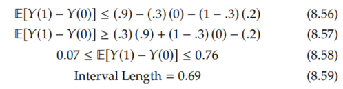
So while the OTS bound 2 from Manski identifies the sign of the ATE in our running example, unlike th OTS bound 1, the OTS bound 2 gives us a 68% larger interval. You can see this by comparing Equation 8.40 (in the above margin) with Equation 8.59.

 

This illustrates some important takeaways:

 

1. Different bounds are better in different cases.

2. Different bounds can be better in different ways (e.g., identifying the sign vs. getting a smaller interval).

Mixing Bounds

Fortunately because both the OTS bound 1 and OTS bound 2 come from the same assumption (Assumption 8.5), we can take the lower bound from OTS bound 2 and the upper bound from OTS bound 1 to get the following tighter interval that still identifies the sign:

 

Similarly, we could have mixed the lower bound from OTS bound 1 and the upper bound from OTS bound 2, but that would have given the worst interval in this subsection for this specific example. It could be the best in a different example, though.

---

8.2. Sensitivity Analysis

8.2.1. Sensitivity Basics in Linear Setting

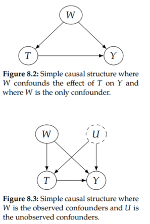
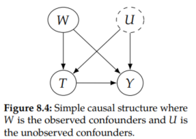
Before this chapter, we have exclusively been working in the setting where causal effects are identifiable. We illustrate the common example of the confounders W as common causes of T and Y in Figure 8.2. In this example, the causal effect of T on Y is identifiable. However, what if there is a single unobserved confounder U, as we illustrate in Figure 8.3. Then, the causal effect is not identifiable.

 

What would be the bias we'd observe if we only adjusted for the observed confounders W? To illustrate this simply, we'll start with a noiseless linear data generating process. So consider data that are generated by the following structural equations:

 

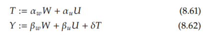
 So the relevant quantity that describes causal effects of T on Y is δ since it is the coefficient in front of T in the structural equation for Y. From the backdoor adjustment (Theorem 4.2) / adjustment formula (Theorem 2.1), we know that

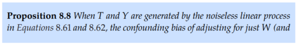
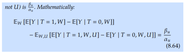
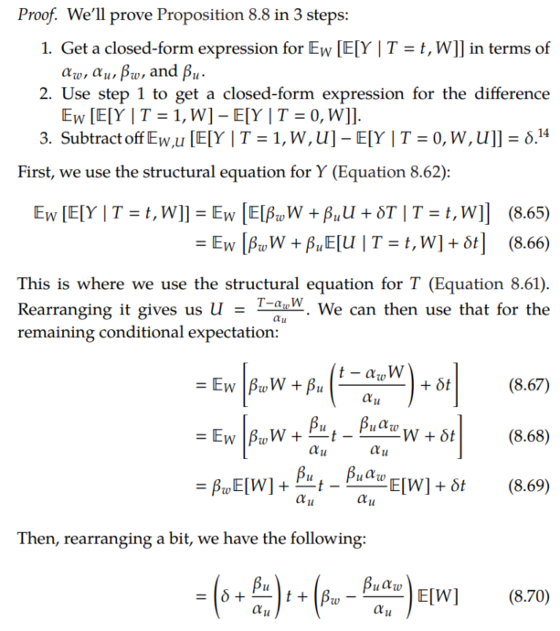
But because U isn't observed, the best we can do is adjust for only W. This leads to a confounding bias of β_u / α_u. We'll be focusing on identification, not estimation, here, so we'll consider that we have infinite data. This means that we hav access to P(W, T, Y). Then, we'll write down and prove the following proposition about confounding bias:

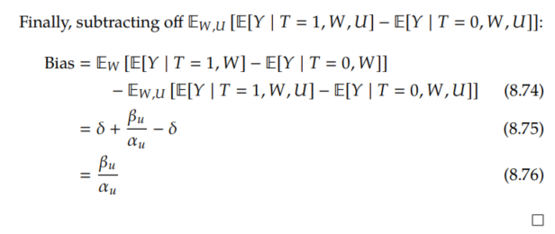
Generalization to Arbitrary Graphs/Estimands

Here, we've performed a sensitivity analysis for the ATE for the simple graph structure in Figure 8.4. For arbitrary estimands in arbitrary graphs, where the structural equations are linear, see Cinelli et al.

Sensitivity Contour Plots

Because Proposition 8.8 gives us a closed-form expression for the bias in terms of the unobserved confounder parameters α_u and β_u, we can plot the levels of bias in contour plots. We show this in Figure 8.5a, where we have 1/ α_u on the x-axis and β_u on the y-axis.

 

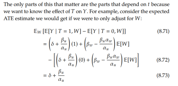
If we rearrange Equation 8.73 to solve for δ, we get the following:

 

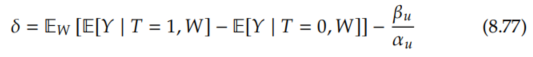
So for given values of α_u and β_u, we can compute the true ATE δ, from the observational quantity Ew[E[Y | T=1, W] - E[Y | T=0, W]]. This allows us to get sensitivity curves that allow us to know how robust conclusions like "Ew[E[Y | T=1, W] - E[Y | T=0, W]] = 25 is positive, so δ is likely positive" are to unobserved confounding. We plot such relevant contours of δ in Figure 8.5b.

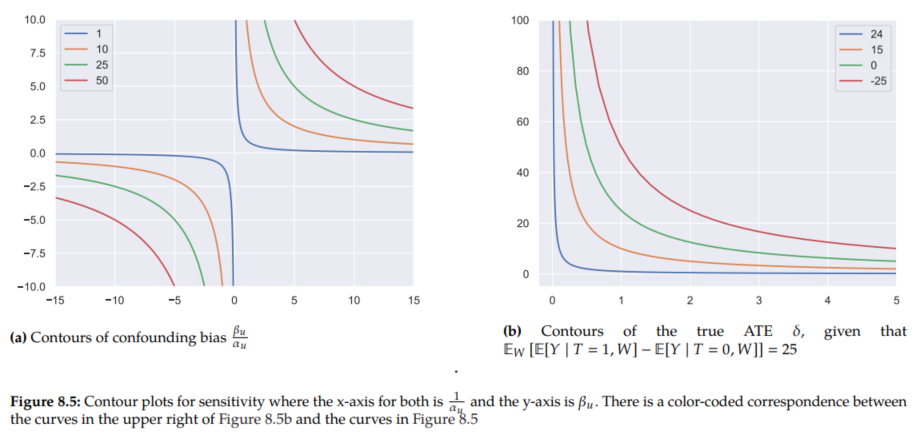
In the example we depict in Figure 8.5, the figure tells us that the green curve (third from the bottom/left) indicates how strong the confounding would need to be in order to completely explain the observed association. In other words, (1/ α_u, β_u) would need to be large enough to fall on the green curve or above in order for the true ATE δ to be zero or the opposite sign of Ew[E[Y | T=1, W] - E[Y | T=0, W]] = 25.

---

8.2.2. More General Settings

We consider a simple linear setting in Section 8.2.1 in order to easily convey the important concepts in sensitivity analysis. However, there is existing that allows us to do sensitivity analysis in more general settings.

 

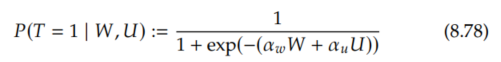
Say we are in the common setting where T is binary. This is not the case in the previous section (Equation 8.61). Rosenbaum and Rubin and Imbens consider a simple binary treatment setting with binary U by just putting a logistic sigmoid function around the right-hand side of Equation 8.61 and using that for the probability of treatment instead of the actual value of treatment:

No Assumptions on T or U

Fortunately, we can drop a lot of the assumptions that we've seen so far. Unlike the linear form that we assumed for T in Section 8.2.1 and the linearish form that Rosenbaum and Rubin and Imbens assume, Cinelli and Hazlett develop a method for sensitivity analysis that is agnostic to the functional form of T. Their method also allows for U to be non-binary and for U to be a vector, rather than just a single unobserved confounder.

Arbitrary Machine Learning Models for Parametrization of T and Y

Recall that all of the estimators that we considered in Chapter 7 allowed us to plug in arbitrary machine learning models to get model-assisted estimators. It might be attractive to have an analogous option in sensitivity analysis, potentially using the exact same models for the conditional outcome model μ and the propensity score e that we used for estimation. And this is exactly what Veitch and Zaveri give us. And they are even able to derive a closed-form expression for confounding bias, assuming the models we use for μ and e are well-specified, something that Rosenbaum and Rubin and Imbens didn't do in their simple setting.

Holy Shit; There are a Lot of Options 

Although we only highlighted a few options above, there are many different approaches to sensitivity analysis, and people don't agree on which ones are best. This means that sensitivity analysis is an active area of current research. 

---