9. Instrumental Variables

https://www.bradyneal.com/causal-inference-course#course-textbook

---

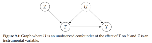
How can we identify causal effects when we are in the presence of unobserved confounding? One popular way is to find and use instrumental variables. An instrument (instrumental variable) Z has three key qualities. 

 

It affects on treatment T, it affects Y only through T, and the effect of Z on Y is unconfounded. We depict these qualities in Figure 9.1. These qualities allow us to use Z to isolate the causal association flowing from T to Y.

 

The intuition is that changes in Z will be reflected in T and lead to corresponding changes in Y. And these specifically Z-focused changes are unconfounded (unlike the changes to T induced by the unobserved confounder U), so they allow us to isolate the causal association that flows from T to Y.

---

9.1. What is an Instrument?

There are three main assumptions that must be satisfied for a variable Z to be considered an instrument. The first is that Z must be relevant in the sense that it must influence T. 

 

Graphically, the relevance assumption corresponds to the existence of an active edge from Z to T in the causal graph. 

 

The second assumption is known as the exclusion restriction.

 

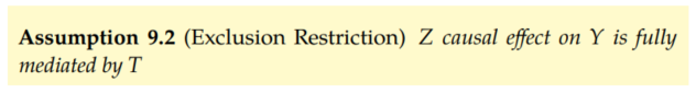
This assumption is known as the exclusion restriction because it excludes Z from the structural equation for Y and from any other structural equations that would make causal association flow from Z to Y without going through T. 

 

Graphically, this means that we've excluded enough potential edges between variables in the causal graph so that all causal paths from Z to Y go through T. 

 

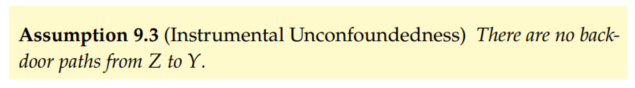
Finally, we assume that the causal effect of Z on Y is unconfounded:

Conditional Instruments

We phrased Assumption 9.3 as unconditional unconfoundedness, but all the math for instrumental variables still works if we have unconfoundedness conditional on observed variables as well. We just have to make sure we condition on those relevant variables. In this case, you might see Z referred to as a conditional instrument.

---

9.2. No Nonparametric Identification of the ATE

You might be wondering "if instrumental variables allow us to identify causal effects, then why didn't we see them back in Chapter 6 Nonparametric Identification?" The answer is that instrumental variables don't nonparametrically identify the causal effect. 

 

We have nonparametric identification when we don't have to make any assumptions about the parametric form. With instrumental variables, we must make assumptions about the parametric form (e.g. linear) to identify causal effects.

 

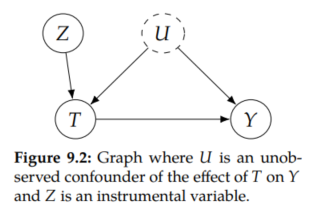
We saw the following useful necessary condition for nonparametric identification in Section 6.3: For each backdoor path from T to any child that is an ancestor of Y, it is possible to block that path. And we can see in Figure 9.2 that there is a backdoor path from T to Y that cannot be blocked: T ←U → Y. So this necessary condition tells us that we can't use the instrument Z to nonparametrically identify the effect of T on Y.

---

9.3. Warm-up: Binary Linear Setting

As a warmp-up, we'll start in the setting where T and Z are binary and where we make the parametric assumption that Y is a linear function of T and U:

 

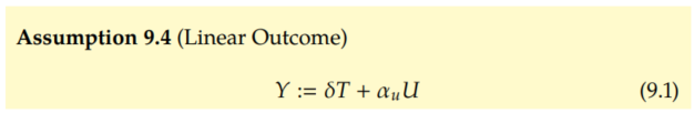
The fact that Z doesn't appear in Equation 9.1 is a consequence of the exclusion restriction (Assumption 9.2).

 

Then, with this assumption in mind, we'll try to identify the causal effect δ. 

 

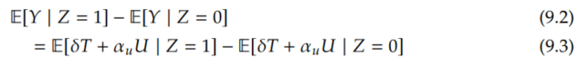
Because we have the intuition that Z will be useful for identifying the effect of T on Y, we'll start with the associational difference for the Z-Y relationship: E[Y | Z=1] - E[Y | Z=0]. By immediately applying Assumption 9.4, we have the following:

 

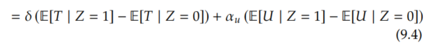
Using linearity of expectation and rearranging a bit:

 

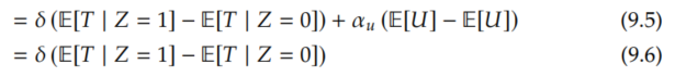
Now, we use the instrumental unconfoundedness assumption (Assumption 9.3). This means that Z and U are independent, which allows us to get rid of the U term:

 

Then, we can solve for δ to get the Wald estimand:

 

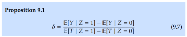
Because of Assumption 9.1, we know that the denominator is non-zero, so the right-hand side isn't undefined. Then, we just plug in empirical means in place of these conditional expectations to get the Wald estimator:

 

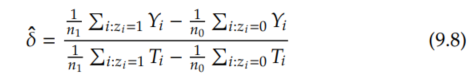
where n1 is the number of samples where Z = 1 and n0 is the number of samples where Z = 0.

Causal Effects as Multiplying Path Coefficients

When the structural equations are linear, you can think of the causal association flowing from a variable A to a variable B as the product of the coefficients along the directed path from A to B. If there are multiple paths, you just sum the causal associations along all those paths. 

 

However, we don't have direct access to the causal association. Rather, we can measure total association, and unblocked backdoor paths also contribute to total association, which is why E[Y | T=1] - E[Y | T=0] ≠ δ.

 

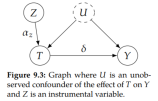
So how can we identify the effect of T on Y in Figure 9.3? Because there are no backdoor paths from the instrument Z to Y, we can trivially identify the effect of Z on Y: E[Y | Z=1] - E[Y | Z=0] = α_z δ. Similarly, we can identify the effect of the instrument on T: E[T | Z=1] - E[T | Z=0] = α_z. Then, we can divide the effect of Z on Y by the effect of the Z on T to identify δ ( α_z δ / α_z). And this quotient is exactly the Wald estimand in Proposition 9.1.

---

9.4. Continuous Linear Setting

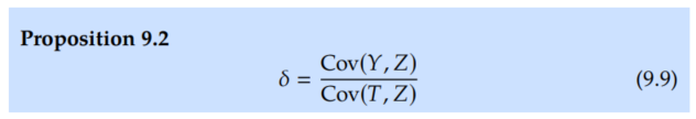
We'll now consider the setting where T and Z are continuous, rather than binary. We'll still assume the linear form for Y (Assumption 9.4), which means that the causal effect of T on Y is δ. In the continuous setting, we get the natural continuous analog of the Wald estimand:

Proof.

Just as we started with E[Y | Z=1] - E[Y | Z=0] in the previous section, here, we'll start with the continuous analog Cov(Y, Z). We start with a classic covariance identity:

 

Then, applying the linear outcome assumption (Assumption 9.4):

 

Distributing and rearranging:

 

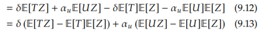
Now, we see that we can apply the same covariance identity again:

 

And Cov(U, Z) = 0 by the instrumental unconfoundedness assumption (Assumption 9.3):

 

Finally, we solve for δ:

 

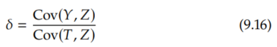
where the relevance assumption (Assumption 9.1) tells us that the denominator is non-zero.

 

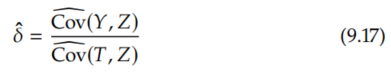
This leads us to the following natural estimator, similar to the Wald estimator:

 

Another equivalent estimator is what's known as the two-stage least squares estimator (2SLS). The two stages are as follows:

 

1. Linearly regress T on Z to estimate E[T | Z]. This gives us the projection of T onto Z: T^.

2. Linearly regress Y on T^ to estimate E[Y | T^]. Obtain our estimate δ^ as the fitted coefficient in front of T^.

 

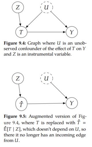
There is helpful intuition that comes with the 2SLS estimator. To see this, start with the canonical instrumental variable graph we've been using (Figure 9.4). In stage one, we are projecting T onto Z to get T^ as a function of only Z: T^ = E^[T | Z]. Then, imagine a graph where T is replaced with T^ (Figure 9.5). Because T^ isn't a function of U, we can think of removing the U → T^ edge in this graph. Now, because there are no backdoor paths from T^ to Y, we can get that association is causation in stage two, where we simply regress Y on T^ to estimate the causal effect. Note: We can also use 2SLS in the binary setting we discussed in Section 9.3.

---

9.5. Nonparametric Identification of Local ATE

The problem with the previous two sections is that we've made the strong parametric assumption of linearity (Assumption 9.4). For example, this assumption requires homogeneity (that the treatment effect is the same for every unit).

 

Ideally, we'd be able to use instrumental variables for identification without making any parametric assumptions such as linearity or homogeneity. And we can. We just need to settle for a more specific causal estimand than the ATE and swap the linearity assumption out for a new assumption. 

 

We will do this in the binary setting, so both T and Z are binary. Before we can do that, we must define a bit of new notation in Section 9.5.1 and introduce principal stratification in Section 9.5.2.

---

9.5.1. New Potential Notation with Instruments

Just like we use Y(1) Δ= Y(T=1) to denote the potential outcome we would observe if we were to take treatment and Y(0) Δ= Y(T=0) to denote the potential outcome we would observe if we were to not take treatment, we will define similar potential notation with instruments.

 

We'll think of the instrument Z as encouragement for the treatment, so if we have Z = 1, we're encouraged to take the treatment, and if we have Z = 0, we're encouraged to not take the treatment. Let T(1) Δ= T(Z=1) denote the treatment we would take if we were to get instrument value 1. Similarly, let T(0) Δ= T(Z=0) denote the treatment we would take if we were to get instrument value 0.

 

Then, we have the same for potential outcomes where we're intervening on the instrument, rather than the treatment: Y(Z=1) denotes the outcome we would observe if we were to be encouraged to take the treatment and Y(Z=0) denotes the outcome we would observe if we were to be encouraged to not take the treatment.

---

9.5.2. Principal Stratification

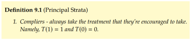
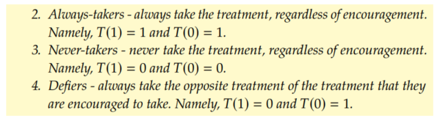
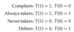
We will segment the population into four principal strata, based on the relationship between the encouragement Z and the treatment taken T. There are four strata because there is one for each combination of the values the binary variables Z and T can take on.

Different Causal Graphs

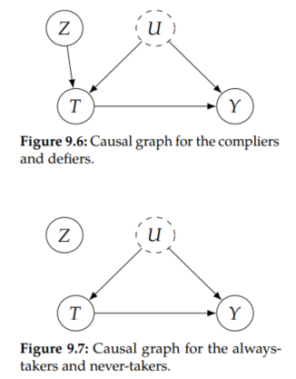
Importantly, these strata have different causal graphs. While the treatment that the compliers and defiers take depends on the encouragement (instrument), the treatment that the always-takers and never-takers take does not. Therefore, the compliers and defiers have the normal causal graph (Figure 9.6), whereas the always-takers and never-takers have the same causal graph but with Z → T edge removed (Figure 9.7). This means that the causal effect of Z on T is zero for always-takers and never takers. Then, because of the exclusion restriction, this means that the causal effect of Z on Y is zero for the always-takers and never takers. This will be important for the upcoming derivation.

Can't Identify Stratum

Given some observed value of Z and T, we can't actually identify which stratum we're in. There are four combinations of the binary variables Z and T; for each of these combinations, we'll note that more than one stratum is compatible with the observed combinations of values.

 

1. Z = 0, T = 0. Compatible strata: compliers or never-takers

2. Z = 0, T = 1. Compatible strata: defiers or always-takers

3. Z =1, T = 0. Compatible strata: defiers or never-takers

4. Z = 1, T = 1. Compatible strata: compliers or always-takers

 

This means that we can't identify if a given unit is a complier, a defier, an always-taker, or a never-taker.

---

9.5.3. Local ATE

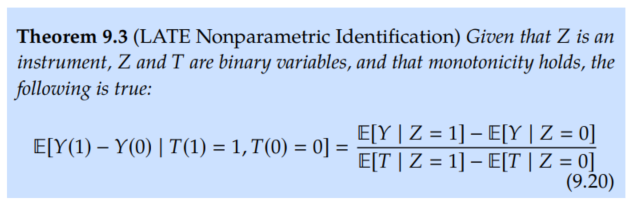
Although we won't be able to use instrumental variables to nonparametrically identify the ATE in the presence of unobserved confounding (Section 9.2), we will be able to nonparametrically identify what's known as the local ATE. 

 

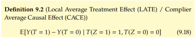
The local average treatment effect (LATE) is also known as the complier average causal effect (CACE), as it is the ATE among the compliers. 

 

To identify the LATE, although we will no longer need the linearity assumption (Assumption 9.4), we will need to introduce a new assumption known as monotonicity.

 

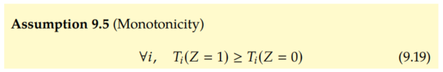
Monotonicity means that if we are encouraged to take treatment (Z = 1), we are either more likely or equally likely to take the treatment than we would be if we were encouraged to not take the treatment (Z = 0). Importantly, this means that we are assuming that there are no defiers. This is because the compliers satisfy T(1) > T(0), the always-takers and never-takers satisfy T(1) = T(0), but the defiers don't satisfy either of these; among the defiers, T(1) < T(0), which is a violation of the monotonicity assumption.

 

We've now introduced the key concept of principal strata and the monotonicity assumption. Importantly, we saw that the causal effect of Z on Y is zero among the always-takers and never-takers, and we just saw that monotonicity assumption implies that there are no defiers. With this in mind, we are now ready to derive the nonparametric identification result for the LATE estimand.

Proof.

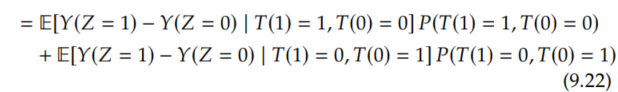
Because we're interested in the causal effect of T on Y and because know that we'll use the instrument Z, we'll start with the causal effect of Z on Y and decompose it into weighted stratum-specific causal effects using the law of total probability:

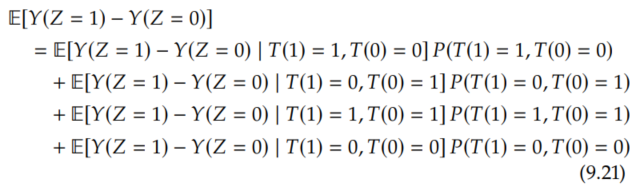
The first term corresponds to the compliers, the second term corresponds to the defiers, the third term corresponds to the always-takers, and the last term corresponds to the never takers. As we discussed, the causal effect of Z on Y among the always-takers and never-takers is zero, so we can remove those terms.

 

Because we've made the monotonicity assumption, we know that there are no defiers (P(T(1)=0,T(0)=1)=0), so the defiers term is also zero.

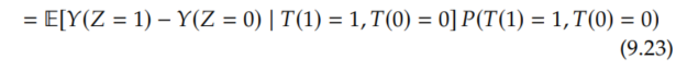
Now, if we solve for this effect of Z on Y among the compliers, we get the following:

 

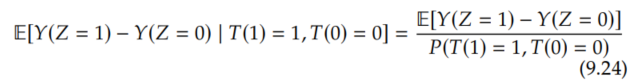
And because these are the compliers, people who will take whichever treatment they are encouraged to take, Y(Z=1) and Y(Z=0) are really equal to Y(T=1) and Y(T=0), respectively, so we can change the left-hand side of Equation 9.24 to the LATE, the causal estimand that we're trying to identify:

 

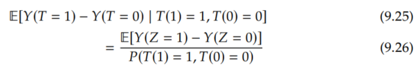
Now, we apply the instrumental unconfoundedness assumption (Assumption 9.3) to identify the numerator.

 

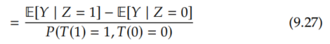
All that's left is to identify the denominator, the probability of being a complier. However, we mentioned that we can't identify the compliers in Section 9.5.2, so how can we do this? This is where we'll need to be a bit clever. We'll get this probability by taking everyone (probability 1) and subtracting out the always-takers and the never-takers, since there are no defiers, due to monotonicity (Assumption 9.5).

 

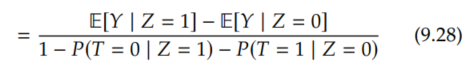
To understand how we got the above equality, consider that everyone either has Z = 1 or Z = 0. We can subtract out all of the never-takers by removing those that had T = 0 among the Z = 1 subpopulation (P(T=0 | Z=1)). Similarly, we can subtract out all of the always-takers by removing those that had T = 1 among the Z = 0 subpopulation (P(T=1 | Z=0)). We know that this removes all of the never-takers and always-takers because there are no defiers and because we've looked at both the Z = 1 subpopulation and the Z = 0 subpopulation. Now, we just do a bit of manipulation:

 

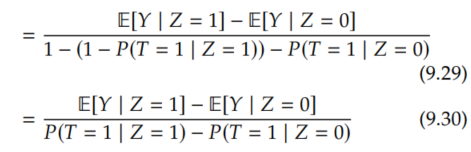
Finally, because T is a binary variable, we can swap out probabilities of T = 1 for expectations:

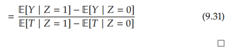
This is exactly the Wald estimand that we saw back in the linear setting (Section 9.3) in Equation 9.7. However, this time, it is the corresponding statistical estimand of the local ATE E[Y(T=1) - Y(T=0) | T(1)=1, T(0)=0], also known as the complier average causal effect (CACE). 

 

This LATE/CACE causal estimand is in contrast to the ATE causal estimand that we saw in Section 9.3: E[Y(T=1) - Y(T=0)]. The difference is that the complier average causal effect is the ATE specifically in the subpopulation of compliers, rather than the total population. It's local (LATE) to that subpopulation, rather than being global over the whole population like the ATE is. So we've seen two different assumptions that get us to the Wald estimand with instrumental variables:

 

1. Linearity (or more generally homogeneity)

2. Monotonicity

Problems with LATE/CACE

There are a few problems with the Wald estimand for LATE, though. The first is that monotonicity might not be satisfied in your setting of interest. The second is that, even if monotonicity is satisfied, you might not be interested in the causal effect specifically among the compliers, especially because you can't even identify who the compliers are. Rather, the regular ATE is often a more useful quantity to know.

---

9.6. More General Settings for ATE Identification

A common more general instrumental variable setting is to consider that the outcome is generated by a complex function of treatment and observed covariates plus some additive unobserved confounders:

See, for example, Hartford et al. and Xu et al. for using deep learning to model f. See references in those papers for using other models such as kernel methods to model f. In those models and given that U enters in the structural equation for Y additively, you can get identification with instrumental variables.

 

Alternatively, we could give up on point identification of causal effects, instead settle for set identification (partial identification), and use instrumental variables to get bounds on causal effects. For more no that, see Pearl. Additionally, settling for identifying a set, rather than a point, allows us to relax the additive noise assumption above in Equation 9.32. For example, Kilbertus et al. considers the setting where U doesn't enter the structural equation for Y additively:

---