10. Causal Discovery from Observational Data

https://www.bradyneal.com/causal-inference-course#course-textbook

---

Throughout this book, we have done causal inference, assuming we know the causal graph. What if we don't know the graph? Can we learn it? As you might expect, based on this being a running theme in this book, it will depend on what assumptions we are willing to make. We will refer to this problem as structure identification, which is distinct from the causal estimand identification that we've seen in the book up until now.

---

10.1. Independence-Based Causal Discovery

10.1.1. Assumptions and Theorem

The main assumption we've seen that relates the graph to the distribution is the Markov assumption. The Markov assumption tells us if variables are d-separated in the graph G, then they are independent in the distribution P (Theorem 3.1):

 

Maybe we can detect independencies in the data and then use that to infer the causal graph. However, going from independencies in the distribution P to d-separations in the graph G isn't something that the Markov assumption gives us (Equation 3.20). Rather, we need the converse of the Markov assumption. This is known as the faithfulness assumption.

 

This assumption allows us to infer d-separations in the graph from independencies in the distribution. Faithfulness, along with the Markov assumption, actually implies minimality (Assumption 3.2), so it is a stronger assumption. 

 

Faithfulness is a much less attractive assumption than the Markov assumption because it is easy to think of counterexamples (where two variables are independent in P, but there are unblocked paths between them in G). 

Faithfulness Counterexample

Consider A and D in the causal graph with coefficients in Figure 11.1. We have a violation of faithfulness when the A → B → D path cancels out the A → C → D path. To concretely see how this could happen, consider the SCM that this graph represents:

 

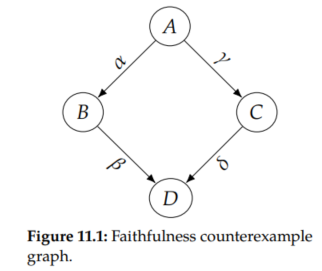
We can solve for the dependence between A and D by plugging in for B and C in Equation 11.4 to get the following:

 

This means that the association flowing from A to D is αβ + γδ in this example. The two paths would cancel if αβ = - γδ, which would make A ㅛ D. This violation of faithfulness would incorrectly lead us to believe that there are no paths between A and D in the graph.

 

In addition to faithfulness, many methods also assume that there are no unobserved confounders, which is known as causal sufficiency.

 

Then, under the Markov, faithfulness, causal sufficiency, and acyclicity assumptions, we can partially identify the causal graph. We can't completely identify the causal graph because different graphs correspond to the same set of independencies. For example, consider the graphs in Figure 11.2.

 

Although these are all distinct graphs, they correspond to the same set of independence/dependence assumptions. Recall from Section 3.5 that X1 ㅛ X3 | X2 in distributions that are Markov with respect to any of these three graphs in Figure 11.2. 

 

We also saw that minimality told us that X1 and X2 are dependent and that X2 and X3 are dependent. And the stronger faithfulness assumption additionally tells us that in any distributions that are faithful with respect to any of these graphs, X1 and X3 are dependent if we don't condition on X2. 

 

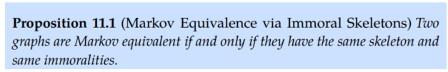
So using the presence/absence of (conditional) independencies in the data isn't enough to distinguish these three graphs from each other; these graphs are Markov equivalent;

 

We say that two graphs are Markov equivalent if they correspond to the same set of conditional independencies. Given a graph, we refer to its Markov equivanlence class as the set of graphs that encode the same conditional independencies. 

 

Under faithfulness, we are able to identify a graph from conditional independencies in the data if it is the only graph in its Marokv equivalence class. Any example of a graph that is the only one in its Markov equivalence class is the basic immorality that we show in Figure 11.3. Recall from Section 3.6 that immoralities are distinct from the two other basic graphical building blocks (chains and forks) in that in Figure 11.3, X1 is (unconditionally) independent of X3, and X1 and X3 become dependent if we condition on X2. This means that while the basic chains and fork in Figure 11.2 are the same Markov equivalence class, the basic immorality is by itself in its own Markov equivalence class.

 

We've seen that se can identify the causal graph if it's a basic immorality, but what else can we identify? We saw that chains and forks are all in the same Markov equivalence class, but that doesn't mean that we can't get any information from distributions that are Markov and faithful with respect to those graphs. What do all the chains and forks in Figure 11.2 have in common? They are share the same skeleton. 

 

A graph's skeleton is the structure we get if we replace all of its directed edges with undirected edges. We depict the skeleton of a basic chain and a basic fork in Figure 11.4.

 

A graph's skeleton also gives us important conditional independence information that we can use to distinguish it from graphs with different skeletons. For example, if we add an X1 → X3 edge to the chain in Figure 11.2a, we get the complete graph Figure 11.5. In this graph, unlike in a chain or fork graph, X1 and X3 are not independent when we condition on X2. So this graph is not in the same Markov equivalence class as the chains and fork in Figure 11.2. 

 

And we can see that graphically by the fact that this graph has a different skeleton than those graphs (this graph has an additional edge between X1 and X3).

 

To recap, we've pointed out two structural qualities that we can use to distinguish graphs from each other:

 

1. Immoralities

2. Skeleton

 

And it turns out that we can determine whether graphs are in the same or different Markov equivalence classes using these two structural qualities, due to a result by Verma and Pearl and Frydenberg.

 

This means that, using conditional independencies in the data, we cannot distinguish graphs that have the same skeletons and same immoralities. For example, we cannot distinguish the two-node graph X → Y from X ← Y using just conditional independence information. But we can hope to learn the graph's skeleton and immoralities; this is known as the essential graph or CPDAG (Completed Partially Directed Acyclic Graph). One popular algorithm for learning the essential graph is the PC algorithm.

---

10.1.2. The PC Algorithm

PC starts with a complete undirected graph and then trims it down and orients edges via three steps:

 

1. Identify the skeleton.

2. Identify immoralities and orient them.

3. Orient qualifying edges that are incident on colliders.

 

We'll use the true graph in Figure 11.6 as a concrete example as we explain each of these steps.

Identify the Skeleton

We discover the skeleton by starting with a complete graph (Figure 11.7a) and then removing edges X - Y where X ㅛ Y | Z for some (potentially empty) conditioning set Z.

 

So in our example, we would start with the empty conditioning set and discover that A ㅛ B (since the only path from A to B in Figure 11.6 is blocked by the collider C); this means we can remove the A - B edge, which gives us the graph in Figure 11.7b. 

 

Then, we would move to conditioning sets of size one and find that conditioning on C tells us that every other pair of variables is conditionally independent given C, which allows us to remove all edges that aren't incident on C, resulting in the graph in Figure 11.7c.

 

And, indeed, this is the skeleton of the true graph in Figure 11.6. More general PC would continue with larger conditioning sets, to see if we can remove more edges, but conditioning sets of size one are enough to discover the skeleton in this example.

 

Identifying the Immoralities

Now for any paths X - Z - Y in our working graph where we discovered that there is no edge between X and Y in our previous step, if Z was not in the conditioning set that makes X and Y conditionally independent, then we know X - Z - Y forms an immorality. 

 

In other words, this means that X ㅛ/ Y | Z, which is a property of an immorality that distinguishes it from chains and forks, so we can orient these edges to get X → Z ← Y. In our example, this takes us from Figure 11.7c to Figure 11.8.

Orienting Qualifying Edges Incident on Colliders

In the final step, we take advantage of the fact that we might be able to orient moer edges since we know we discovered all of the immoralities in the previous step. Any edge Z - Y part of a partially directed path of the form X → Z - Y, where there is no edge connecting X and Y, can be oriented as Z → Y.

 

This is because if the true graph has the edge Z ← Y, we would have found this in the previous step as that would have formed an immorality X → Z ← Y. Since we didn't find that immorality in the previous step, we know that the true direction is Z → Y. In our example, this means we can orient the final two remaining edges, taking us from Figure 11.8 to Figure 11.9. 

 

It turns out that in this example, we are lucky that we can orient all of the remaining edges in this last step, but this is not the case in general. For example, we discussed that we wouldn't be able to distinguish simple chain graphs and simple fork graphs from each other.

 

Dropping Assumptions

There are algorithms that allow us to drop various assumptions. The FCI (Fast Causal Inference) algorithm works without assuming causal sufficiency (Assumption 11.2). The CCD algorithm works without assuming acyclicity. And there is various work on SAT-based causal discovery that allows us to drop both of the above assumptions.

Hardness of Conditional Independence Testing

All methods that rely on conditional independence tests such as PC, FCI, SAT-based algorithm, etc. have an important practical issue associated with them. Conditional independence tests are hard, and it can sometimes require a lot of data to get accurate test results. If we have infinite data, this isn't an issue, but we don't have infinite data in practice.

---

10.1.3. Can we Get Any Better Identification?

We've seen that assuming the Markov assumption and faithfulness can only get us so far; with those assumptions, we can only identify a graph up to its Markov equivalence class. If we make more assumptions, can we identify the graph more precisely than just its Markov equivalence class?

 

If we are in the case where the distributions are multinomial, we cannot. Or if we are in the common toy case where the SCMs are linear with Gaussian noise, we cannot. So we have the following completeness result due to Geiger and Pearl and Meek:

 

What if we don't have multinomial distributions and don't have linear Gaussian SCMs, though?

---

10.2. Semi-Parametric Causal Discovery

In Theorem 11.2, we saw that, if we are in the linear Gaussian setting, the best we can do is identify the Markov equivalence class; we cannot hope to identify graphs that are in non-singleton Markov equivalence classes. But what if we aren't in the linear Gaussian setting? Can we identify graphs if we are not in the linear Gaussian setting?

 

We consider the linear non-Gaussian noise setting in Section 10.2.2 and the nonlinear additive noise setting in Section 10.2.3. It turns out that in both of these settingss, we can identify the causal graph. And we don't have to assume faithfulness (Assumption 11.1) in these settings.

 

By considering these settings, we are making semi-parametric assumptions (about functional form). If we don't make any assumptions about functional form, we cannot even identify the direction of the edge in a two-node graph. We emphasize this in the next section before moving on to the semi-parametric assumptions that allow us to identify the graph.

---

10.2.1. No Identifiability Without Parametric Assumptions

Markov Perspective

Consider the two-variable setting, where the two options of causal graphs are X → Y and X ← Y. Note that these two graphs are Markov equivalent. Both don't encode any conditional independence assumptions, so both can describe arbitrary distributions P(x, y). 

 

This means that conditional independencies in the data cannot help us distinguish between X → Y and X ← Y. Using conditional independencies, the best we cao do is discover the corresponding essential graph X - Y.

SCMs Perspective

How about if we consider this problem from the perspective of SCMs; can we somehow distinguish X → Y from X ← Y using SCMs? For an SCM, we want to write one variable as a function of the other variable and some noise term variable. As you might expect, if we don't make any assumptions, there exist SCMs with the implied causal graph X → Y and SCMs with the implied causal graph X ← Y that both generate data according to P(x, y).

 

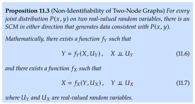
Similarly, this non-identifiability result can be extended to more general graphs that have more than two variables.

 

However, if we make assumptions about the parametric form of the SCM, we can distinguish X → Y from X ← Y and identify graphs more generally. That's what we'll see in the rest of this chapter.

---

10.2.2. Linear Non-Gaussian Noise

We saw in Theorem 11.2 that we cannot distinguish graphs within the same Markov equivalence class if the structural equations are linear with Gaussian noise U. For example, this means that we cannot distinguish X → Y from X ← Y. 

 

However, if the niose term is non-Gaussian, then we can identify the causal graph. 

 

Then, in this linear non-Gaussian setting, we can identify which of graphs X → Y and X ← Y is the true causal graph. We'll first present the theorem and proof and then get to the intuition.

Proof.

We'll first introduce a important result from Darmois and Skitovich that we'll use to prove this theorem:

 

We will use the contrapositive of the special case of this theorem for n = 2 to do almost all of the work for this proof:

Proof Outline

With the above corollary in mind, our proof strategy is to write Y and U~ as linear combinations of X and U. By doing this, we are effectively mapping our variables in Equation 11.9 and 11.10 onto the variables in the corollary as follows: Y onto A, U~ onto B, X onto X1, and U onto X2. 

 

Then, we can apply the above corollary of the Darmois-Skitovich Theorem to have that Y and U~ must be dependent, which violates the reverse direction SCM in Equation 11.10. We now proceed with the proof.

 

We already have that we can write Y as a linear combination of X and U, since we've assumed the true structural equation in Equation 11.9 is linear:

 

Then, to get U~ as a linear combination of X and U, we take the hypothesized reverse SCM

 

from Equation 11.10, solve for U~, and plug in Equation 11.11 for Y:

 

Therefore, we've written both Y and U~ as linear combinations of the independent random variables X and U. This allows us to apply Corollary 11.6 of the Darmois-Skitovish Theorem to get that Y and U~ must be dependent: Y ㅛ/ U~. This violates the reverse direction SCM:

We've given the proof here for just two variables, but it can be extended to the more general setting with multiple variables.

Graphical Intuition

When we fit the data in the causal direction, we get residuals that are independent of the input variable, but when we fit the data in the anti-causal direction, we get residuals that are dependent on the input variable. 

 

We depict the regression line f^ we get if we linearly regress Y on X (causal direction) in Figure 11.10a, and we depict the regression line g^ we get if we linearly regress X on Y (anti-causal direction) in Figure 11.10b. Just from these fits, you can see that the forward model (fit in the causal direction) looks more pleasing than the backward model (fit in the anti-causal direction).

 

To make this graphical intuition more clear, we plot the residuals of the forward model f^ (causal direction) and the backward model g^ (anti-causal direction) in Figure 11.11. The residuals in the forward direction correspond to the following: U^ = Y - f^(X). And the residuals in the backward direction correspond to the following: U~^ = X - g^(Y). As you can see in Figure 11.11a, the residuals of the forward model look independent of the input variable X (on the x-axis). However in Figure 11.10b, the residuals of the backward model don't look independent of the input variable Y (on the x-axis) at all. Clearly, the range of the residuals (on the vertical) changes as we move across values of Y (from left to right).

---

10.2.3. Nonlinear Models

Nonlinear Additive Noise Setting

We can also get identifiability of the causal graph in the nonlinear additive noise setting. This requires the nonlinear additive noise assumption (below) and other more technical assumptions that we refer you to Hoyer et al. and Peters et al. for.

Post-Nonlinear Setting

What if you don't believe that the noise realistically enters additively. This motivates post-nonlinear models, where there is another nonlinear transformation after adding the noise as in Assumption 11.5 below. This setting can also yield identifiability (under another technical condition).

---