Normalizing Flows Tutorial, Part 1: Distributions and Determinants

https://blog.evjang.com/2018/01/nf1.html

---

If you are a machine learning practitioner working on generative modeling, Bayesian deep learning, or deep reinforcement learning, normalizing flows are a handy technique to have in your algorithmic toolkit. Normalizing flows transform simple densities (like Gaussians) into rich complex distributions that can be used for generative models, RL, and variational inference. 

 

This tutorial comes in two parts:

• Part 1: Distributions and Determinants. In this post, I explain how invertible transformations of densities can be used to implement more complex densities, and how these transformations can be chained together to form a “normalizing flow”.
• Part 2: Modern Normalizing Flows: In a follow-up post, I survey recent techniques developed by researchers to learn normalizing flows, and explain how a slew of modern generative modeling techniques -- autoregressive models, MAF, IAF, NICE, Real-NVP, Parallel-Wavenet -- are all related to each other.

 

---

Background

Statistical Machine Learning algorithms try to learn the structure of data by fitting a parametric distribution p(x;θ) to it. Given a dataset, if we can represent it with a distribution, we can:

1. Generate new data “for free” by sampling from the learned distribution in silico; no need to run the true generative process for the data. This is a useful tool if the data is expensive to generate, i.e. a real-world experiment that takes a long time to run [1]. Sampling is also used to construct estimators of high-dimensional integrals over spaces.
2. Evaluate the likelihood of data observed at test time (this can be used for rejection sampling or to score how good our model is).
3. Find the conditional relationship between variables. For example, learning the distribution p(x2|x1) allows us to build discriminative classification or regression models.
4. Score our algorithm by using complexity measures like entropy, mutual information, and moments of the distribution.

We've gotten pretty good at sampling (1), as evidenced by recent work on generative models for images and audio. These kinds of generative models are already being deployed in real commercial applications and Google products. 

 

However, the research community currently directs less attention towards unconditional & conditional likelihood estimation (2, 3) and model scoring (4). For instance, we don’t know how to compute the support of a GAN decoder (how much of the output space has been assigned nonzero probability by the model), we don’t know how to compute the density of an image with respect to a DRAW distribution or even a VAE, and we don’t know how to analytically compute various metrics (KL, earth-mover distance) on arbitrary distributions, even if we know their analytic densities.

 

Generating likely samples isn’t enough: we also care about answering “how likely is the data?” [2], having flexible conditional densities (e.g. for sampling/evaluating divergences of multi-modal policies in RL), and being able to choose rich families of priors and posteriors in variational inference. 

 

Consider for a moment, your friendly neighborhood Normal Distribution. It’s the Chicken Soup of distributions: we can draw samples from it easily, we know its analytic density and KL divergence to other Normal distributions, the central limit theorem gives us confidence that we can apply it to pretty much any data, and we can even backprop through its samples via the reparameterization trick. The Normal Distribution’s ease-of-use makes it a very popular choice for many generative modeling and reinforcement learning algorithms.

 

Unfortunately, the Normal distribution just doesn’t cut it in many real-world problems we care about. In Reinforcement Learning -- especially continuous control tasks such as robotics -- policies are often modeled as multivariate Gaussians with diagonal covariance matrices. 

 

By construction, uni-modal Gaussians cannot do well on tasks that require sampling from a multi-modal distribution. A classic example of where uni-modal policies fail is an agent trying to get to its house across a lake. It can get home by circumventing the lake clockwise (left) or counterclockwise (right), but a Gaussian policy is not able to represent two modes. Instead, it chooses actions from a Gaussian whose mean is a linear combination of the two modes, resulting in the agent going straight into the icy water. Sad!

 

The above example illustrates how the Normal distribution can be overly simplistic. In addition to bad symmetry assumptions, Gaussians have most of their density concentrated at the edges in high dimensions and are not robust to rare events. Can we find a better distribution with the following properties?

1. Complex enough to model rich, multi-modal data distributions like images and value functions in RL environments?
2. ... while retaining the easy comforts of a Normal distribution: sampling, density evaluation, and with re-parameterizable samples?

The answer is yes! Here are a few ways to do it:

• Use a mixture model to represent a multi-modal policy, where a categorical represents the “option” and the mixture represents the sub-policy. This provides samples that are easy to sample and evaluate, but samples are not trivially re-parameterizable, which makes them hard to use for VAEs and posterior inference. However, using a Gumbel-Softmax / Concrete relaxation of the categorical “option” would provide a multi-modal, re-parameterizable distribution.
• Autoregressive factorizations of policy / value distributions. In particular,  the Categorical distribution can model any discrete distribution.
• In RL, one can avoid this altogether by symmetry-breaking the value distribution via recurrent policies, noise, or distributional RL. This helps by collapsing the complex value distributions into simpler conditional distributions at each timestep. 
• Learning with energy-based models, a.k.a undirected graphical models with potential functions that eschew an normalized probabilistic interpretation. Here’s a recent example of this applied to RL.
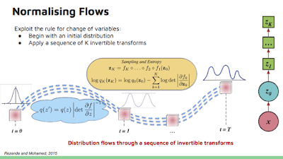
• Normalizing Flows: learn invertible, volume-tracking transformations of distributions that we can manipulate easily.

Let's explore the last approach - Normalizing Flows.

---

Change of Variables, Change of Volume

Let's build up some intuition by examining linear transformations of 1D random variables. Let X be the distribution Uniform(0,1). Let random variable Y=f(X)=2X+1. Y is a simple affine (scale & shift) transformation of the underlying “source distribution” X. What this means is that a sample xi from X can be converted into a sample from Y by simply applying the function f to it. 

The green square represents the shaded probability mass on R for both p(x) and p(y) - the height represents the density function at that value. Observe that because probability mass must integrate to 1 for any distribution, the act of scaling the domain by 2 everywhere means we must divide the probability density by 2 everywhere, so that the total area of the green square and blue rectangle are the same (=1).

 

If we zoom in on a particular x and an infinitesimally nearby point x+dx, then applying f to them takes us to the pair (y,y+dy).

 

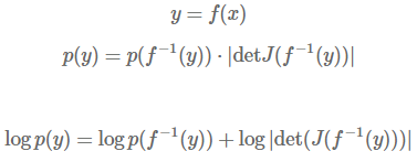
On the left, we have a locally increasing function (dy/dx>0) and on the right, a locally decreasing function (dy/dx<0). In order to preserve total probability, the change of p(x) along interval dx must be equivalent to the change of p(y) along interval dy:

In order to conserve probability, we only care about the amount of change in y and not its direction (it doesn’t matter if f(x) is increasing or decreasing at x, we assume the amount of change in y is the same regardless). Therefore, p(y)=p(x)|dx/dy|. Note that in log-space, this is equivalent to logp(y)=logp(x)+log|dx/dy|. Computing log-densities is more well-scaled for numerical stability reasons.

 

Now let’s consider the multivariate case, with 2 variables. Again, zooming into an infinitesimally small region of our domain, our initial “segment” of the base distribution is now a square with width dx.

 

Note that a transformation that merely shifts a rectangular patch (x1,x2,x3,x4) does not change the area. We are only interested in the rate of change per unit area of x, so the displacement dx can be thought of as a unit of measure, which is arbitrary. To make the following analysis simple and unit-less, let’s investigate a unit square on the origin, i.e. 4 points (0,0),(1,0),(0,1),(1,1).

 

Multiplying this by the matrix [[a,b];[c,d]] will take points on this square into a parallelogram, as shown on the figure to the right (below). (0,0) is sent to (0,0), (1,0) is sent to (a,b), (1,0) sent to (c,d), (1,1) sent to (a+c,b+d).

Thus, a unit square in the domain of X corresponds to a deformed parallelogram in the domain of Y, so the per-unit rate of change in area is the area of the parallelogram, i.e. ad−bc.

 

The area of a parallelogram, ad−bc, is nothing more than the absolute value of the determinant of the linear transformation!

 

In 3 dimensions, the “change in area of parallelogram” becomes a “change in volume of parallelpiped”, and even higher dimensions, this becomes “change in volume of a n-parallelotope”. But the concept remains the same - determinants are nothing more than the amount (and direction) of volume distortion of a linear transformation, generalized to any number of dimensions.

 

What if the transformation f is nonlinear? Instead of a single parallelogram that tracks the distortion of any point in space, you can picture many infinitesimally small parallelograms corresponding to the amount of volume distortion for each point in the domain. Mathematically, this locally-linear change in volume is |det(J(f−1(x)))|, where J(f^-1(x)) is the Jacobian of the function inverse - a higher-dimensional generalization of the quantity dx/dy from before.

When I learned about determinants in middle & high school I was very confused at the seemingly arbitrary definition of determinants. We were only taught how to compute a determinant, instead of what a determinant meant: the local, linearized rate of volume change of a transformation.

---

Normalizing Flows and Learning Flexible Bijectors

Why stop at 1 bijector? We can chain any number of bijectors together, much like we chain layers together in a neural network [3]. This is construct is known as a “normalizing flow”. Additionally, if a bijector has tunable parameters with respect to bijector.log_prob, then the bijector can actually be learned to transform our base distribution to suit arbitrary densities. Each bijector functions as a learnable “layer”, and you can use an optimizer to learn the parameters of the transformation to suit our data distribution we are trying to model. One algorithm to do this is maximum likelihood estimation, which modifies our model parameters so that our training data points have maximum log-probability under our transformed distribution. We compute and optimize over log probabilities rather than probabilities for numerical stability reasons.

 

However, computing the determinant of an arbitrary N×N Jacobian matrix has runtime complexity O(N^3), which is very expensive to put in a neural network. There is also the trouble of inverting an arbitrary function approximator. Much of the current research on Normalizing Flows focuses on how to design expressive Bijectors that exploit GPU parallelism during forward and inverse computations, all while maintaining computationally efficient ILDJs.