Making LLMs even more accessible with bitsandbytes, 4-bit quantization and QLoRA

https://huggingface.co/blog/4bit-transformers-bitsandbytes

---

LLMs are known to be large, and running or training them in consumer hardware is a huge challenge for users and accessibility. Our LLM.int8 blogpost showed how the techniques in the LLM.int8 paper were integrated in transformers using the bitsandbytes library. As we strive to make models even more accessible to anyone, we decided to collaborate with bitsandbytes again to allow users to run models in 4-bit precision. This includes a large majority of HF models, in any modality (text, vision, multi-modal, etc.). Users can also train adapters on top of 4bit models leveraging tools from the Hugging Face ecosystem. This is a new method introduced today in the QLoRA paper by Dettmers et al. The abstract of the paper is as follows:

 

"We present QLoRA, an efficient finetuning approach that reduces memory usage enough to finetune a 65B parameter model on a single 48GB GPU while preserving full 16-bit finetuning task performance. QLoRA backpropagates gradients through a frozen, 4-bit quantized pretrained language model into Low Rank Adapters~(LoRA). Our best model family, which we name Guanaco, outperforms all previous openly released models on the Vicuna benchmark, reaching 99.3% of the performance level of ChatGPT while only requiring 24 hours of finetuning on a single GPU. QLoRA introduces a number of innovations to save memory without sacrificing performance: (a) 4-bit NormalFloat (NF4), a new data type that is information theoretically optimal for normally distributed weights (b) double quantization to reduce the average memory footprint by quantizing the quantization constants, and (c) paged optimizers to manage memory spikes. We use QLoRA to finetune more than 1,000 models, providing a detailed analysis of instruction following and chatbot performance across 8 instruction datasets, multiple model types (LLaMA, T5), and model scales that would be infeasible to run with regular finetuning (e.g. 33B and 65B parameter models). Our results show that QLoRA finetuning on a small high-quality dataset leads to state-of-the-art results, even when using smaller models than the previous SoTA. We provide a detailed analysis of chatbot performance based on both human and GPT-4 evaluations showing that GPT-4 evaluations are a cheap and reasonable alternative to human evaluation. Furthermore, we find that current chatbot benchmarks are not trustworthy to accurately evaluate the performance levels of chatbots. A lemon-picked analysis demonstrates where Guanaco fails compared to ChatGPT. We release all of our models and code, including CUDA kernels for 4-bit training."

---

Resources

This blogpost and release come with several resources to get started with 4bit models and QLoRA:

• Original paper
• Basic usage Google Colab notebook - This notebook shows how to use 4bit models in inference with all their variants, and how to run GPT-neo-X (a 20B parameter model) on a free Google Colab instance 🤯
• Fine tuning Google Colab notebook - This notebook shows how to fine-tune a 4bit model on a downstream task using the Hugging Face ecosystem. We show that it is possible to fine tune GPT-neo-X 20B on a Google Colab instance!
• Original repository for replicating the paper's results
• Guanaco 33b playground - or check the playground section below

---

Introduction

If you are not familiar with model precisions and the most common data types (float16, float32, bfloat16, int8), we advise you to carefully read the introduction in our first blogpost that goes over the details of these concepts in simple terms with visualizations.

 

For more information we recommend reading the fundamentals of floating point representation through this wikibook document.

 

The recent QLoRA paper explores different data types, 4-bit Float and 4-bit NormalFloat. We will discuss here the 4-bit Float data type since it is easier to understand.

 

FP8 and FP4 stand for Floating Point 8-bit and 4-bit precision, respectively. They are part of the minifloats family of floating point values (among other precisions, the minifloats family also includes bfloat16 and float16).

 

Let’s first have a look at how to represent floating point values in FP8 format, then understand how the FP4 format looks like.

FP8 format

As discussed in our previous blogpost, a floating point contains n-bits, with each bit falling into a specific category that is responsible for representing a component of the number (sign, mantissa and exponent). These represent the following.

 

The FP8 (floating point 8) format has been first introduced in the paper “FP8 for Deep Learning” with two different FP8 encodings: E4M3 (4-bit exponent and 3-bit mantissa) and E5M2 (5-bit exponent and 2-bit mantissa).

Overview of Floating Point 8 (FP8) format. Source: Original content from sgugger

Although the precision is substantially reduced by reducing the number of bits from 32 to 8, both versions can be used in a variety of situations. Currently one could use Transformer Engine library that is also integrated with HF ecosystem through accelerate.

 

The potential floating points that can be represented in the E4M3 format are in the range -448 to 448, whereas in the E5M2 format, as the number of bits of the exponent increases, the range increases to -57344 to 57344 - but with a loss of precision because the number of possible representations remains constant. It has been empirically proven that the E4M3 is best suited for the forward pass, and the second version is best suited for the backward computation

FP4 precision in a few words

The sign bit represents the sign (+/-), the exponent bits a base two to the power of the integer represented by the bits (e.g. 2^{010} = 2^{2} = 4), and the fraction or mantissa is the sum of powers of negative two which are “active” for each bit that is “1”. If a bit is “0” the fraction remains unchanged for that power of 2^-i where i is the position of the bit in the bit-sequence. For example, for mantissa bits 1010 we have (0 + 2^-1 + 0 + 2^-3) = (0.5 + 0.125) = 0.625. To get a value, we add 1 to the fraction and multiply all results together, for example, with 2 exponent bits and one mantissa bit the representations 1101 would be:

 

-1 * 2^(2) * (1 + 2^-1) = -1 * 4 * 1.5 = -6

 

For FP4 there is no fixed format and as such one can try combinations of different mantissa/exponent combinations. In general, 3 exponent bits do a bit better in most cases. But sometimes 2 exponent bits and a mantissa bit yield better performance.

---

QLoRA paper, a new way of democratizing quantized large transformer models

In few words, QLoRA reduces the memory usage of LLM finetuning without performance tradeoffs compared to standard 16-bit model finetuning. This method enables 33B model finetuning on a single 24GB GPU and 65B model finetuning on a single 46GB GPU.

 

More specifically, QLoRA uses 4-bit quantization to compress a pretrained language model. The LM parameters are then frozen and a relatively small number of trainable parameters are added to the model in the form of Low-Rank Adapters. During finetuning, QLoRA backpropagates gradients through the frozen 4-bit quantized pretrained language model into the Low-Rank Adapters. The LoRA layers are the only parameters being updated during training. Read more about LoRA in the original LoRA paper.

 

QLoRA has one storage data type (usually 4-bit NormalFloat) for the base model weights and a computation data type (16-bit BrainFloat) used to perform computations. QLoRA dequantizes weights from the storage data type to the computation data type to perform the forward and backward passes, but only computes weight gradients for the LoRA parameters which use 16-bit bfloat. The weights are decompressed only when they are needed, therefore the memory usage stays low during training and inference.

 

QLoRA tuning is shown to match 16-bit finetuning methods in a wide range of experiments. In addition, the Guanaco models, which use QLoRA finetuning for LLaMA models on the OpenAssistant dataset (OASST1), are state-of-the-art chatbot systems and are close to ChatGPT on the Vicuna benchmark. This is an additional demonstration of the power of QLoRA tuning.

---

How to use it in transformers?

In this section let us introduce the transformers integration of this method, how to use it and which models can be effectively quantized.

Getting started

As a quickstart, load a model in 4bit by (at the time of this writing) installing accelerate and transformers from source, and make sure you have installed the latest version of bitsandbytes library (0.39.0).

pip install -q -U bitsandbytes
pip install -q -U git+https://github.com/huggingface/transformers.git
pip install -q -U git+https://github.com/huggingface/peft.git
pip install -q -U git+https://github.com/huggingface/accelerate.git

Quickstart

The basic way to load a model in 4bit is to pass the argument load_in_4bit=True when calling the from_pretrained method by providing a device map (pass "auto" to get a device map that will be automatically inferred).

from transformers import AutoModelForCausalLM

model = AutoModelForCausalLM.from_pretrained("facebook/opt-350m", load_in_4bit=True, device_map="auto")
...

 

That's all you need!

 

As a general rule, we recommend users to not manually set a device once the model has been loaded with device_map. So any device assignment call to the model, or to any model’s submodules should be avoided after that line - unless you know what you are doing.

 

Keep in mind that loading a quantized model will automatically cast other model's submodules into float16 dtype. You can change this behavior, (if for example you want to have the layer norms in float32), by passing torch_dtype=dtype to the from_pretrained method.

Advanced usage

You can play with different variants of 4bit quantization such as NF4 (normalized float 4 (default)) or pure FP4 quantization. Based on theoretical considerations and empirical results from the paper, we recommend using NF4 quantization for better performance.

 

Other options include bnb_4bit_use_double_quant which uses a second quantization after the first one to save an additional 0.4 bits per parameter. And finally, the compute type. While 4-bit bitsandbytes stores weights in 4-bits, the computation still happens in 16 or 32-bit and here any combination can be chosen (float16, bfloat16, float32 etc).

 

The matrix multiplication and training will be faster if one uses a 16-bit compute dtype (default torch.float32). One should leverage the recent BitsAndBytesConfig from transformers to change these parameters. An example to load a model in 4bit using NF4 quantization below with double quantization with the compute dtype bfloat16 for faster training:

from transformers import BitsAndBytesConfig


nf4_config = BitsAndBytesConfig(
   load_in_4bit=True,
   bnb_4bit_quant_type="nf4",
   bnb_4bit_use_double_quant=True,
   bnb_4bit_compute_dtype=torch.bfloat16
)

model_nf4 = AutoModelForCausalLM.from_pretrained(model_id, quantization_config=nf4_config)

 

Changing the compute dtype

As mentioned above, you can also change the compute dtype of the quantized model by just changing the bnb_4bit_compute_dtype argument in BitsAndBytesConfig.

import torch
from transformers import BitsAndBytesConfig

quantization_config = BitsAndBytesConfig(
   load_in_4bit=True,
   bnb_4bit_compute_dtype=torch.bfloat16
)

Nested quantization

For enabling nested quantization, you can use the bnb_4bit_use_double_quant argument in BitsAndBytesConfig. This will enable a second quantization after the first one to save an additional 0.4 bits per parameter. We also use this feature in the training Google colab notebook.

from transformers import BitsAndBytesConfig

double_quant_config = BitsAndBytesConfig(
   load_in_4bit=True,
   bnb_4bit_use_double_quant=True,
)

model_double_quant = AutoModelForCausalLM.from_pretrained(model_id, quantization_config=double_quant_config)

 

And of course, as mentioned in the beginning of the section, all of these components are composable. You can combine all these parameters together to find the optimial use case for you. A rule of thumb is: use double quant if you have problems with memory, use NF4 for higher precision, and use a 16-bit dtype for faster finetuning. For instance in the inference demo, we use nested quantization, bfloat16 compute dtype and NF4 quantization to fit gpt-neo-x-20b (40GB) entirely in 4bit in a single 16GB GPU.

---

Common questions

Does FP4 quantization have any hardware requirements?

Note that this method is only compatible with GPUs, hence it is not possible to quantize models in 4bit on a CPU. Among GPUs, there should not be any hardware requirement about this method, therefore any GPU could be used to run the 4bit quantization as long as you have CUDA>=11.2 installed. Keep also in mind that the computation is not done in 4bit, the weights and activations are compressed to that format and the computation is still kept in the desired or native dtype.

What are the supported models?

Similarly as the integration of LLM.int8 presented in this blogpost the integration heavily relies on the accelerate library. Therefore, any model that supports accelerate loading (i.e. the device_map argument when calling from_pretrained) should be quantizable in 4bit. Note also that this is totally agnostic to modalities, as long as the models can be loaded with the device_map argument, it is possible to quantize them.

 

For text models, at this time of writing, this would include most used architectures such as Llama, OPT, GPT-Neo, GPT-NeoX for text models, Blip2 for multimodal models, and so on.

 

At this time of writing, the models that support accelerate are:

[
    'bigbird_pegasus', 'blip_2', 'bloom', 'bridgetower', 'codegen', 'deit', 'esm', 
    'gpt2', 'gpt_bigcode', 'gpt_neo', 'gpt_neox', 'gpt_neox_japanese', 'gptj', 'gptsan_japanese', 
    'lilt', 'llama', 'longformer', 'longt5', 'luke', 'm2m_100', 'mbart', 'mega', 'mt5', 'nllb_moe', 
    'open_llama', 'opt', 'owlvit', 'plbart', 'roberta', 'roberta_prelayernorm', 'rwkv', 'switch_transformers', 
    't5', 'vilt', 'vit', 'vit_hybrid', 'whisper', 'xglm', 'xlm_roberta'
]

Can we train 4bit/8bit models?

It is not possible to perform pure 4bit training on these models. However, you can train these models by leveraging parameter efficient fine tuning methods (PEFT) and train for example adapters on top of them. That is what is done in the paper and is officially supported by the PEFT library from Hugging Face. We also provide a training notebook and recommend users to check the QLoRA repository if they are interested in replicating the results from the paper.

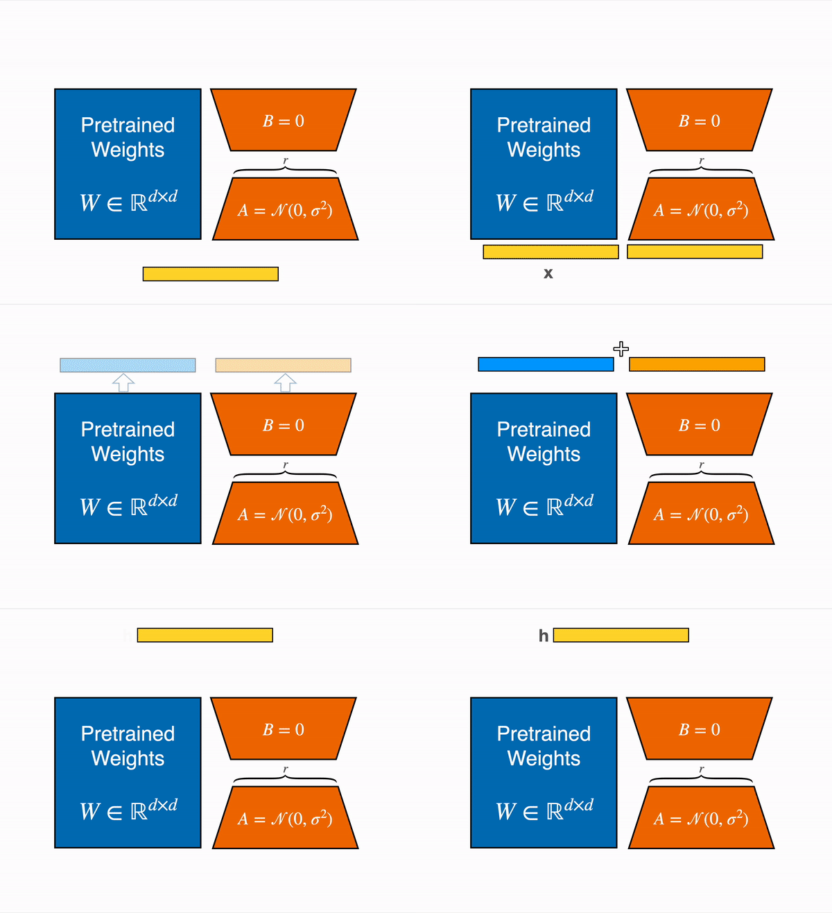
The output activations original (frozen) pretrained weights (left) are augmented by a low rank adapter comprised of weight matrics A and B (right).

---

8-bit Matrix Multiplication for transformers at scale using Hugging Face Transformers, Accelerate and bitsandbytes

Common data types used in Machine Learning

We start with the basic understanding of different floating point data types, which are also referred to as "precision" in the context of Machine Learning.

 

The size of a model is determined by the number of its parameters, and their precision, typically one of float32, float16 or bfloat16

Float32 (FP32) stands for the standardized IEEE 32-bit floating point representation. With this data type it is possible to represent a wide range of floating numbers. In FP32, 8 bits are reserved for the "exponent", 23 bits for the "mantissa" and 1 bit for the sign of the number. In addition to that, most of the hardware supports FP32 operations and instructions.

 

In the float16 (FP16) data type, 5 bits are reserved for the exponent and 10 bits are reserved for the mantissa. This makes the representable range of FP16 numbers much lower than FP32. This exposes FP16 numbers to the risk of overflowing (trying to represent a number that is very large) and underflowing (representing a number that is very small).

 

For example, if you do 10k * 10k you end up with 100M which is not possible to represent in FP16, as the largest number possible is 64k. And thus you'd end up with NaN (Not a Number) result and if you have sequential computation like in neural networks, all the prior work is destroyed. Usually, loss scaling is used to overcome this issue, but it doesn't always work well.

 

A new format, bfloat16 (BF16), was created to avoid these constraints. In BF16, 8 bits are reserved for the exponent (which is the same as in FP32) and 7 bits are reserved for the fraction.

 

This means that in BF16 we can retain the same dynamic range as FP32. But we lose 3 bits of precision with respect to FP16. Now there is absolutely no problem with huge numbers, but the precision is worse than FP16 here.

 

In the machine learning jargon FP32 is called full precision (4 bytes), while BF16 and FP16 are referred to as half-precision (2 bytes). On top of that, the int8 (INT8) data type consists of an 8-bit representation that can store 2^8 different values (between [0, 255] or [-128, 127] for signed integers).

 

While, ideally the training and inference should be done in FP32, it is two times slower than FP16/BF16 and therefore a mixed precision approach is used where the weights are held in FP32 as a precise "main weights" reference, while computation in a forward and backward pass are done for FP16/BF16 to enhance training speed. The FP16/BF16 gradients are then used to update the FP32 main weights.

 

During training, the main weights are always stored in FP32, but in practice, the half-precision weights often provide similar quality during inference as their FP32 counterpart -- a precise reference of the model is only needed when it receives multiple gradient updates. This means we can use the half-precision weights and use half the GPUs to accomplish the same outcome.

To calculate the model size in bytes, one multiplies the number of parameters by the size of the chosen precision in bytes. For example, if we use the bfloat16 version of the BLOOM-176B model, we have 176*10**9 x 2 bytes = 352GB! As discussed earlier, this is quite a challenge to fit into a few GPUs.

 

But what if we can store those weights with less memory using a different data type? A methodology called quantization has been used widely in Deep Learning.

---

Introduction to model quantization

Experimentially, we have discovered that instead of using the 4-byte FP32 precision, we can get an almost identical inference outcome with 2-byte BF16/FP16 half-precision, which halves the model size. It'd be amazing to cut it further, but the inference quality outcome starts to drop dramatically at lower precision.

 

To remediate that, we introduce 8-bit quantization. This method uses a quarter precision, thus needing only 1/4th of the model size! But it's not done by just dropping another half of the bits.

 

Quantization is done by essentially “rounding” from one data type to another. For example, if one data type has the range 0..9 and another 0..4, then the value “4” in the first data type would be rounded to “2” in the second data type. However, if we have the value “3” in the first data type, it lies between 1 and 2 of the second data type, then we would usually round to “2”. This shows that both values “4” and “3” of the first data type have the same value “2” in the second data type. This highlights that quantization is a noisy process that can lead to information loss, a sort of lossy compression.

 

The two most common 8-bit quantization techniques are zero-point quantization and absolute maximum (absmax) quantization. Zero-point quantization and absmax quantization map the floating point values into more compact int8 (1 byte) values. First, these methods normalize the input by scaling it by a quantization constant.

 

For example, in zero-point quantization, if my range is -1.0…1.0 and I want to quantize into the range -127…127, I want to scale by the factor of 127 and then round it into the 8-bit precision. To retrieve the original value, you would need to divide the int8 value by that same quantization factor of 127. For example, the value 0.3 would be scaled to 0.3*127 = 38.1. Through rounding, we get the value of 38. If we reverse this, we get 38/127=0.2992 – we have a quantization error of 0.008 in this example. These seemingly tiny errors tend to accumulate and grow as they get propagated through the model’s layers and result in performance degradation.

 

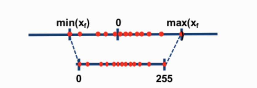
Now let's look at the details of absmax quantization. To calculate the mapping between the fp16 number and its corresponding int8 number in absmax quantization, you have to first divide by the absolute maximum value of the tensor and then multiply by the total range of the data type.

 

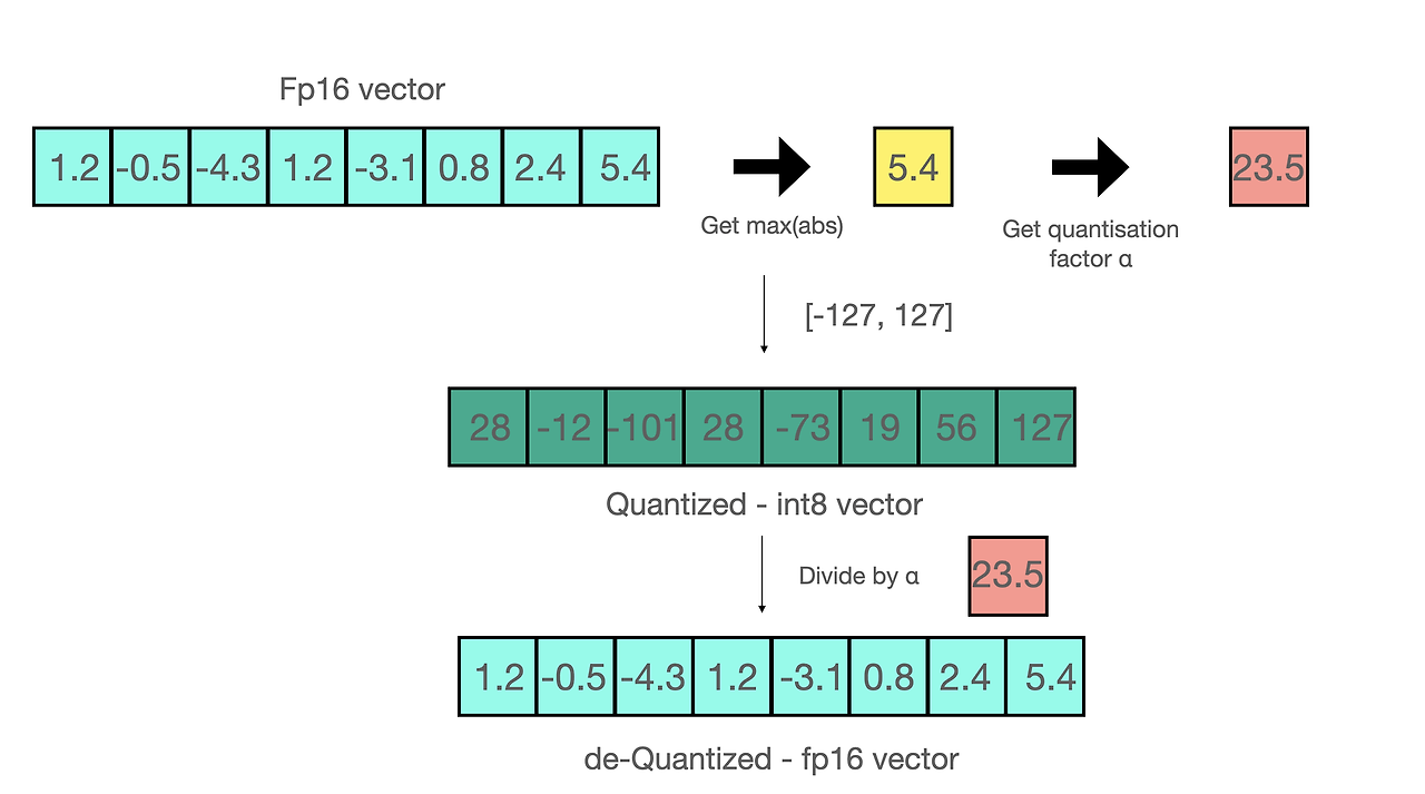
For example, let's assume you want to apply absmax quantization in a vector that contains [1.2, -0.5, -4.3, 1.2, -3.1, 0.8, 2.4, 5.4]. You extract the absolute maximum of it, which is 5.4 in this case. Int8 has a range of [-127, 127], so we divide 127 by 5.4 and obtain 23.5 for the scaling factor. Therefore multiplying the original vector by it gives the quantized vector [28, -12, -101, 28, -73, 19, 56, 127].

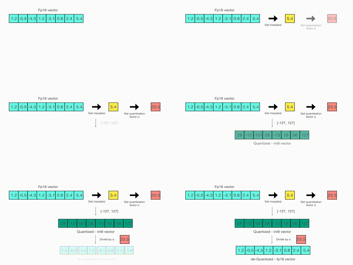
To retrieve the latest, one can just divide in full precision the int8 number with the quantization factor, but since the result above is "rounded" some precision will be lost.

 

For an unsigned int8, we would subtract the minimum and scale by the absolute maximum. This is close to what zero-point quantization does. It's is similar to a min-max scaling but the latter maintains the value scales in such a way that the value “0” is always represented by an integer without any quantization error.

 

These tricks can be combined in several ways, for example, row-wise or vector-wise quantization, when it comes to matrix multiplication for more accurate results. Looking at the matrix multiplication, A*B=C, instead of regular quantization that normalize by a absolute maximum value per tensor, vector-wise quantization finds the absolute maximum of each row of A and each column of B. Then we normalize A and B by dividing these vectors. We then multiply A*B to get C. Finally, to get back the FP16 values, we denormalize by computing the outer product of the absolute maximum vector of A and B. More details on this technique can be found in the LLM.int8() paper or in the blog post about quantization and emergent features on Tim's blog.

 

While these basic techniques enable us to quanitize Deep Learning models, they usually lead to a drop in accuracy for larger models. The LLM.int8() implementation that we integrated into Hugging Face Transformers and Accelerate libraries is the first technique that does not degrade performance even for large models with 176B parameters, such as BLOOM.

---

A gentle summary of LLM.int8(): zero degradation matrix multiplication for Large Language Models

In LLM.int8(), we have demonstrated that it is crucial to comprehend the scale-dependent emergent properties of transformers in order to understand why traditional quantization fails for large models. We demonstrate that performance deterioration is caused by outlier features, which we explain in the next section. The LLM.int8() algorithm itself can be explain as follows.

 

In essence, LLM.int8() seeks to complete the matrix multiplication computation in three steps:

 

1. From the input hidden states, extract the outliers (i.e. values that are larger than a certain threshold) by column.
2. Perform the matrix multiplication of the outliers in FP16 and the non-outliers in int8.
3. Dequantize the non-outlier results and add both outlier and non-outlier results together to receive the full result in FP16.

These steps can be summarized in the following animation:

 

The importance of outlier features

A value that is outside the range of some numbers' global distribution is generally referred to as an outlier. Outlier detection has been widely used and covered in the current literature, and having prior knowledge of the distribution of your features helps with the task of outlier detection. More specifically, we have observed that classic quantization at scale fails for transformer-based models >6B parameters. While large outlier features are also present in smaller models, we observe that a certain threshold these outliers from highly systematic patterns across transformers which are present in every layer of the transformer. For more details on these phenomena see the LLM.int8() paper and emergent features blog post.

 

As mentioned earlier, 8-bit precision is extremely constrained, therefore quantizing a vector with several big values can produce wildly erroneous results. Additionally, because of a built-in characteristic of the transformer-based architecture that links all the elements together, these errors tend to compound as they get propagated across multiple layers. Therefore, mixed-precision decomposition has been developed to facilitate efficient quantization with such extreme outliers. It is discussed next.

Inside the MatMul

Once the hidden states are computed we extract the outliers using a custom threshold and we decompose the matrix into two parts as explained above. We found that extracting all outliers with magnitude 6 or greater in this way recoveres full inference performance. The outlier part is done in fp16 so it is a classic matrix multiplication, whereas the 8-bit matrix multiplication is done by quantizing the weights and hidden states into 8-bit precision using vector-wise quantization -- that is, row-wise quantization for the hidden state and column-wise quantization for the weight matrix. After this step, the results are dequantized and returned in half-precision in order to add them to the first matrix multiplication.

What does 0 degradation mean?

How can we properly evaluate the performance degradation of this method? How much quality do we lose in terms of generation when using 8-bit models?

 

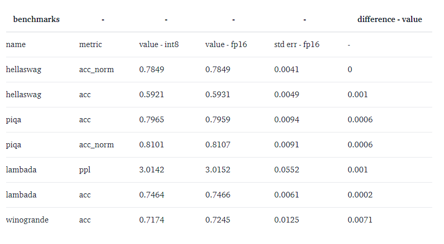
We ran several common benchmarks with the 8-bit and native models using lm-eval-harness and reported the results.

 

For OPT-175B:

For BLOOM-176:

 

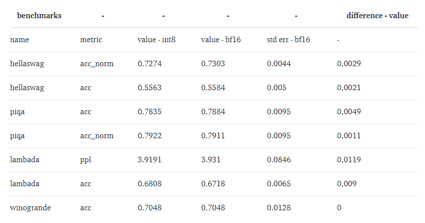
We indeed observe 0 performance degradation for those models since the absolute difference of the metrics are all below the standard error (except for BLOOM-int8 which is slightly better than the native model on lambada). For a more detailed performance evaluation against state-of-the-art approaches, take a look at the paper!

Is it faster than native models?

The main purpose of the LLM.int8() method is to make large models more accessible without performance degradation. But the method would be less useful if it is very slow. So we benchmarked the generation speed of multiple models. We find that BLOOM-176B with LLM.int8() is about 15% to 23% slower than the fp16 version – which is still quite acceptable. We found larger slowdowns for smaller models, like T5-3B and T5-11B. We worked hard to speed up these small models. Within a day, we could improve inference per token from 312 ms to 173 ms for T5-3B and from 45 ms to 25 ms for T5-11B. Additionally, issues were already identified, and LLM.int8() will likely be faster still for small models in upcoming releases. For now, the current numbers are in the table below.

 

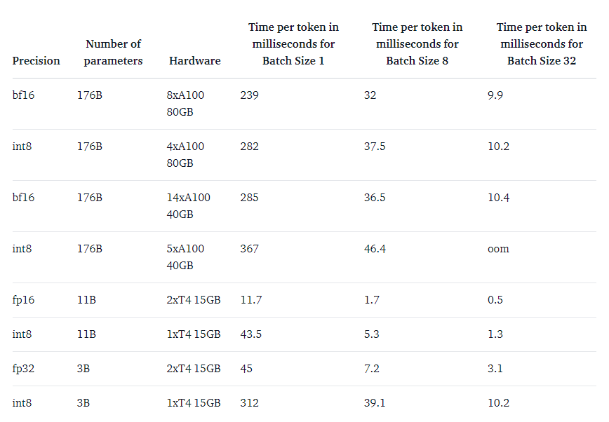
The 3 models are BLOOM-176B, T5-11B and T5-3B.

---