-
CLIP - Creating strong image and language representations for general machine learning tasks.Research/Multimodal 2024. 9. 26. 11:39
https://towardsdatascience.com/clip-intuitively-and-exhaustively-explained-1d02c07dbf40
CLIP - Creating strong image and language representations for general machine learning tasks.
In this post you’ll learn about “contrastive language-image pre-training” (CLIP), A strategy for creating vision and language representations so good they can be used to make highly specific and performant classifiers without any training data. We’ll go over the theory, how CLIP differs from more conventional methods, then we’ll walk through the architecture step by step.
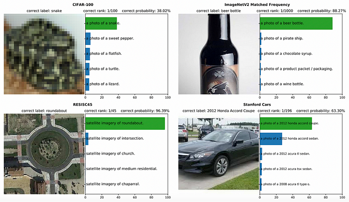
CLIP predicting highly specific labels for classification tasks it was never directly trained on. Source
The Typical Image Classifier
When training a model to detect if an image is of a cat or a dog, a common approach is to present a model with images of both cats and dogs, then incrementally adjust the model based on it’s errors until it learns to distinguish between the two.
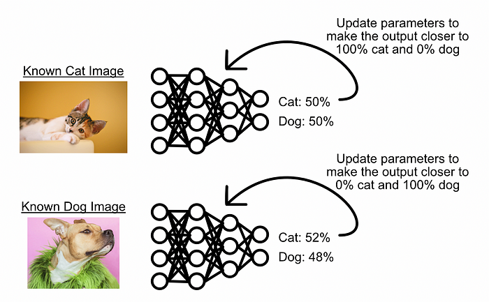
A conceptual diagram of what supervised learning might look like. Imagine we have a new model which doesn’t know anything about images. We can feed it an image, ask it to predict the class of the image, then update the parameters of the model based on how wrong it is. We can then do this numerous times until the model starts performing well at the task. I explore back propagation in this post , which is the mechanism which makes this generally possible. This traditional form of supervised learning is perfectly acceptable for many use cases, and is known to perform well in a variety of tasks. However, this strategy is also known to result in highly specialized models which only perform well within the bounds of their initial training.

Comparing CLIP with a more traditional supervised model. Each of the models were trained on and perform well on ImageNet (a popular image classification dataset), but when exposed to similar datasets containing the same classes in different representations, the supervised model experiences a large degradation in performance, while CLIP does not. This implies that the representations in CLIP are more robust and generalizable than other methods. Source To resolve the issue of over-specialization, CLIP approaches classification in a fundamentally different way; by trying to learn the association between images and their annotation through contrastive learning. We’ll explore what that means in the next section.
CLIP, in a Nutshell
What if, instead of creating a model that can predict if an image belongs to one of some list of classes, we create a model which predicts if an image belongs to some arbitrary caption? This is a subtle shift in thinking which opens the doors to completely new training strategies and model applications.

The end result of CLIP, a model which can predict if some arbitrary text belongs with an arbitrary image The core idea of CLIP is to use captioned images scraped from the internet to create a model which can predict if text is compatible with an image or not.

An example of CLIP applied to various data sets it hasn’t seen before. While not completely perfect (it predicted the wrong type of aeroplane), CLIP displays a remarkable ability to understand a variety of different classification problems out of the box. Source CLIP does this by learning how to encode images and text in such a way that, when the text and image encodings are compared to each other, matching images have a high value and non-matching images have a low value. In essence, the model learns to map images and text into a landscape such that matching pairs are close together, and not matching pairs are far apart. This strategy of learning to predict if things belong or don’t belong together is commonly referred to as “contrastive learning”.

A conceptual diagram of contrastive learning from the perspective of CLIP. In essence, we put every image and every caption in some arbitrary space. We then learn to place those images and captions within that space such that matching pairs are close together, and non-matching pairs are far apart. In CLIP, contrastive learning is done by learning a text encoder and an image encoder, which learns to put an input into some position in a vector space. CLIP then compares these positions during training and tries to maximize the closeness of positive pairs, and minimize the closeness of negative pairs.

A diagram of CLIP. We take a bunch of images and their corresponding description and learn how to encode them such that matching values are large, and not matching values are small. In the diagram above the blue highlighted region corresponds to positive matching pairs, and the rest of the matrix corresponds to negative pairs which need to be minimized. Source The general strategy CLIP employs allows us to do all sorts of things:
- We can build image classifiers by just asking the model which text, like “a photo of a cat” and “a photo of a dog” are most likely to be associated with an image
- We can build an image search system which can be used to find the image which is most related to input text. For instance, we can look at a variety of images and find which image is most likely to correspond to the text “a photo of a dog”
- We can use the image encoder by itself to extract abstract information about an image which is relevant to text. The encoder can position images in space dependent on the content of the image, that information can be used by other machine learning models.
- We can use the text encoder by itself to extract abstract information about text which is relevant to images. The encoder can position text in space dependent on the entire content of the text, that information can be used by other machine learning models.

Recall that we’re learning to position images and text in such a way that similar things are close together. In doing this process we’ve found a way to put both text and images in meaningful locations. To do this effectively we have to build encoders which have a strong understanding of images and text. We need to be able to understand “catness” in an image, or understand that the word “fabulous” is modifying the word “jacket”. As a result, the encoders used in CLIP can be used in isolation to be able to extract meaning from certain inputs. While zero-shot classification is pretty cool (zero-shot meaning the ability to perform well on an unseen type of data. For instance, asking the model “is this person happy” when it was never trained explicitly to detect happiness), extracting and using just the text or image encoder within CLIP has become even more popular. Because CLIP models are trained to create subtle and powerful encodings of text and images which can represent complex relationships, the high quality embeddings from the CLIP encoders can be co-opted for other tasks;
I have an article which uses the image encoder from CLIP to enable language models to understand images, for instance:
So, now we have a high level understanding of CLIP. Don’t worry if you don’t completely understand; in the next section we’ll break down CLIP component by component to build an intuitive understanding of how it functions.
So, now we have a high level understanding of CLIP. Don’t worry if you don’t completely understand; in the next section we’ll break down CLIP component by component to build an intuitive understanding of how it functions.
The Components of CLIP
CLIP is a high level architecture which can use a variety of different sub components to achieve the same general results. We’ll be following the CLIP paper and break down one of the possible approaches.
The text Encoder

The Text Encoder within CLIP, source At its highest level, the text encoder converts input text into a vector (a list of numbers) that represents the text’s meaning.

The purpose of a text encoder, essentially The text encoder within CLIP is a standard transformer encoder. For the purposes of this article, a transformer can be thought of as a system which takes an entire input sequence of words, then re-represents and compares those words to create an abstract, contextualized representation of the entire input. The self attention mechanism within a transformer is the main mechanism that creates that contextualized representation.
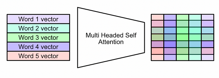
Multi Headed Self Attention, the main operation in a transformer, takes an input sequence of words and converts them into an abstract representation. The end result can be conceptualized as containing “contextualized meaning” rather than a list of words. One modification CLIP makes to the general transformer strategy is that it results in a vector, not a matrix, which is meant to represent the entire input sequence. It does this by simply extracting the vector for the last token in the input sequence. This works because the self attention mechanism is designed to contextualize each input with every other input. Thus, after passing through multiple layers of self attention, the transformer can learn to encode all necessary meaning into a single vector.

A conceptual diagram of CLIP’s text encoder; multiple multi-headed self attention layers manipulating the output into a final vector which represents the entire input. This final vector is used to represent the text input as a point in space, which is ultimately used to calculate the “closeness” between a caption and an image. In the next section we’ll talk about Image encoders, which convert an image into a representative vector.
The Image Encoder

The Image Encoder within CLIP, source At its highest level, the image encoder converts an image into a vector (a list of numbers) that represents the images meaning.

The purpose of an image encoder, essentially There are a few approaches to image encoders which are discussed in the CLIP paper. In this article we’ll consider ResNET-50, a time tested convolutional approach which has been applied to several general image tasks. I’ll be covering ResNET in a future post, but for the purposes of this article we can just think of ResNET as a classic convolutional neural network.
A convolutional neural network is a strategy of image modeling which filters an image with a small matrix of values called a kernel. It sweeps the kernel through the image and calculates a new value for each pixel based on the kernel and the input image.
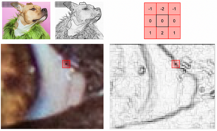
A conceptual diagram of transforming an image via a Kernel. The kernel is placed in a certain spot within an image and multiplies the surrounding pixels by some value. It then adds those multiplied values together to calculate a new value for the image at that location. The values of each kernel are learnable, and a convolutional network uses many kernels. The end result is a network which learns to re-represent an input numerous different ways to extract meaning from an image. The whole idea behind a convolutional network is, by doing a combination of convolutions and downsampling of an image, you can extract more and more subtle feature representations. Once an image has been condensed down to a small number of high quality abstract features, a dense network can then be used to turn those features into some final output. I talk about this more in depth in another post, specifically the role of the dense network at the end, called a projection head.

A classic convolutional architecture from the YOLO paper, an landmark object detection model. Each of these boxes describe an input images horizontal and vertical size, as well as their “depth”, in terms of number of features. The input image is an RGB image, so it has a depth of 3. The following box has a “depth” of 192, which corresponds to having 192 kernels extracting different information from the input image. By extracting more and more features, and downsampling the image via maxpooling, the network distills the image into an abstract representation which is trained to hold some meaning about the image. Source From the perspective of CLIP, the end result ends up being a vector which can be thought of as a summary of the input image. This vector, along with the summary vectors for text, are then used in the next section to construct a multi-modal embedding space, which we’ll discuss in the next section.

The image encoder used in CLIP in a nutshell. The image encoder converts an image into an abstract set of features with a convolutional network, then uses a dense, fully connected neural network to create the final output. In this case, the final output vector can be thought of as a summary of the entire input
The Multi-Modal Embedding Space, and CLIP Training
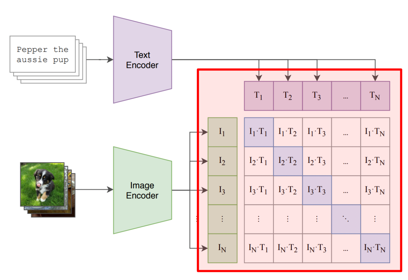
The component of the CLIP training process which jointly aligns the embedding for both text and images In the previous two sections we went over modeling strategies which can summarize text and images into vectors. In this section we’ll go over how CLIP uses those vectors to build strong image and language representations.

The image and text encoder “embedding” each input. Note: the length of these embeddings is typically very long, maybe 256 elements long. We can think of these embedding vectors as representing the input as some point in high dimensional space. For demonstrative purposes we can imagine creating encoders which embed their input into a vector of length two. These vectors could then be considered as points in a two dimensional space, and we could draw their positions.

an example of CLIP before it’s trained, with 2 dimensional embeddings for demonstrative purposes. Each of the images is passed through the image encoder to create a vector of length 2, and each of the input text is passed through the text encoder to create a vector of length 2 We can think of this space as the Multi-Modal Embedding Space, and we can train CLIP (by training the image and text encoders) to put these points in spots such that positive pairs are close to each other.

an example of CLIP after it’s trained, with 2 dimensional embeddings for demonstrative purposes. Notice how, once the encoders are trained, positive pairs end up close together There are a lot of ways to define “close” in machine learning. Arguably the most common approach is cosine similarity, which is what CLIP employs. The idea behind cosine similarity is that we can say two vectors are similar if the angle between them is small.

If calculating similarity based on cosine similarity, the angle between A and B is small, and thus A and B are similar. C would be considered very different from both A and B The term “cosine” comes from the cosine function, a trigonometry function which calculates the ratio of the adjacent leg of a right triangle with the hypotenuse based on some angle. If that sounds like gibberish, no big deal: if the angle is small between two vectors, the cosine between the two vectors will be close to 1. If the vectors are 90 degrees apart, the cosine will be zero. If the vectors are pointing in opposite directions, the cosine will be -1. As a result, with cosine, you get big numbers when the vectors point in the same direction, and you get small numbers when they don't.

A conceptual diagram for how the cosine wave (the wave on the bottom) relates to the anglue within a right triangle. It’s really not that important to understand the cosine function completely for this article, only that it’s biggest when the angle between things is 0, and smallest when things point in opposite directions. If you’re curious about learning more about trigonometry and waves, you can refer to this article I wrote on how frequency analysis relates to machine learning The cosine of the angle between two vectors can be calculated by measuring the angle between them and then passing that angle through the cosine function. Printing out all the vectors and measuring the angle between them using a protractor might slow down our training time, though. Luckily, we can use the following identity to calculate the cosine of the angle between two vectors:
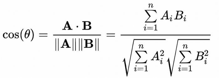
If you were already daunted by math, you might feel even more daunted now. But I’ll break it down:
- The phrase A•B represents the dot product between vector A and B. The dot product is what you get when you multiply every element in A by the corresponding element in B, then sum all the results. So if A=[1,2,3], and B=[2,3,4], then A•B = (1x2) + (2x3) + (3x4).
- The phrase “||(some vector)||”, as in ||A|| or ||B||, represents the calculation of the norm of a vector. This is simply the magnitude, or length, of the vector. The length of a vector can be calculated by taking the square root of the sum of squares in a vector. So, for A=[1,2,3], ||A|| = sqrt(1² + 2² + 3²)
- You can, conceptually, think of the numerator A•B as the similarity, while the denominator ||A||||B|| divides the similarity by the lengths of the vectors. This division makes the cosine similarity only change based on the angle between vectors, and not their size. Without the denominator reigning things in, A•B would be bigger if A and B got longer, regardless of their direction.
If we look back at our original diagram, we might notice that we’re calculating dot products between the embedding of images and text

The calculation of distance between image and text representations in CLIP. notice how the dot product, the numerator of the cosine similarity, is calculated between each embedding for text and images Because of the way loss is calculated, all the image and text vectors will have a length of 1 and, as a result, we can forgo dividing by the magnitude of the vectors. So, while we’re not dividing by the denominator, this is still conceptually trained using cosine similarity (we’ll touch on this more in the next section).
Now that we have an idea of how we go from image and text to embedding vectors, and how those embedding vectors get used to calculate similarity, we can look a bit more in-depth at how training practically shakes out by exploring how CLIP uses contrastive loss.
CLIP and contrastive loss
The whole idea of contrastive loss is, instead of looking at individual examples to try to boost performance on a per-pair basis, you can instead think of the problem as incrementally improving the closeness of positive pairs while, simultaneously, preserving the distance of negative pairs.
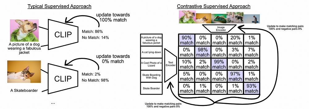
A traditional supervised approach on the left, and contrastive approach on the right. The supervised approach works on individual input-output pairs (usually in the form of a mini-batch, but still a grouping of one to one pairs), while the contrastive approach pairs every possible pair together and tries to raise the closeness of positive pairs (highlighted in blue) and reduce the closeness of negative pairs. In CLIP this is done by computing the dot product between the encoded text and image representations which, as we discussed previously, can be used to quantify “closeness”.
This shift in thinking towards contrastive learning is really what makes CLIP so powerful. There are a lot of ways the caption for an image can be generated; a picture can be captioned “A cat lying down”, “feline relaxing”, “little cutie george taking a nap”, whatever. It’s difficult to predict the actual caption of an image, but by using “closeness” and “farness”, CLIP can deal with this problem elegantly.
CLIP uses 32,768 image-text pairs every single batch, which is a pretty big batch size compared to a more traditional approach which might see a batch size of 16–64. As a result, CLIP is forced to be really good at getting positive pairs far away from a large number of negative pairs, which is what makes CLIP so robust.
in order to train a neural network you need a single value for performance, called the “loss”, which you can use to update the model. Each training step you update the model’s parameters such that the model would output a smaller loss value at that step. The CLIP paper includes the following pseudo code which describes how loss is calculated within CLIP:
# image_encoder - ResNet or Vision Transformer
# text_encoder - CBOW or Text Transformer
# I[n, h, w, c] - minibatch of aligned images
# T[n, l] - minibatch of aligned texts
# W_i[d_i, d_e] - learned proj of image to embed
# W_t[d_t, d_e] - learned proj of text to embed
# t - temperature parameter

# 1) get a batch of aligned images and text
I, T = get_mini_batch()

# 2) extract feature representations of each modality
I_f = image_encoder(I) #[n, d_i]
T_f = text_encoder(T) #[n, d_t]

# 3) joint multimodal embedding [n, d_e]
I_e = l2_normalize(np.dot(I_f, W_i), axis=1)
T_e = l2_normalize(np.dot(T_f, W_t), axis=1)

# 4) scaled pairwise cosine similarities [n, n]
logits = np.dot(I_e, T_e.T) * np.exp(t)

# 5) symmetric loss function
labels = np.arange(n)
loss_i = cross_entropy_loss(logits, labels, axis=0)
loss_t = cross_entropy_loss(logits, labels, axis=1)
loss = (loss_i + loss_t)/2
Breaking this down into components:
- First we get a batch of images of dimension [batch size, image height, image width, number of colors] and a batch of text of dimension [batch size, sequence length]. These batches are aligned with each other, such that every image in the batch of images corresponds with every piece of text in the batch of text.
- We pass these through our encoder, which results in some vector for each image and each piece of text in their respective batches.
- In order for the images and text to be placed in the same embedding space, the vectors are passed through a linear projection. This can be thought of as a single layer dense network without biases or an activation function. The CLIP paper talks about how the details of this aren’t super important, just that both image and text vectors end up being the same length. These vectors are normalized using l2 normalization, which keeps the vectors pointing in the same direction but compresses all vectors to a length of one.
- Because all embedding vectors are of length 1, there’s no need to divide by their magnitude to calculate cosine similarity. Thus, the dot product between the embedding vectors is equivalent to cosine similarity. The cosine similarity is multiplied by a temperature parameter, which controls how intensely the similarities effect a given training epoch.
- loss is calculated across text and images symmetrically via cross entropy loss. This is mentioned offhandedly in the CLIP paper, but the details can be a bit tricky.
In researching for this article, I found the following expression for cross entropy loss:
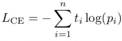
Cross entropy loss, where “t” is the value of some true label and “p” is the value of some prediction This idea is all well and good, but cosin similarity goes from -1 to 1 as we previously discussed, and you can’t take the log of a negative number. The CLIP paper mentions the following:
The cosine similarity of these embeddings is then calculated, scaled by a temperature parameter τ , and normalized into a probability distribution via a softmax. — CLIP
Using this information, as well as information from the pseudo code:
# 5) symmetric loss function
# logits = nxn matrix of cosin similarity predictions
# labels = nxn matrix of true values
labels = np.arange(n)
loss_i = cross_entropy_loss(logits, labels, axis=0)
loss_t = cross_entropy_loss(logits, labels, axis=1)
loss = (loss_i + loss_t)/2
We can infer that the cross_entropy_loss function (as a function specified in the pseudo code) contains a softmax operation over the specified axis. This is a fiddly detail, but it’s important in making CLIP train effectively.
For those who might not be aware, a softmax function takes a vector of some values and turns it into a positive vector with a sum of components equal to one.

The softmax function. The use of exp has all sorts of nice properties, but essentially the softmax function squashes down an input vector such that elements in the vector are between 0 and 1, and the sum of all elements in the vector is 1 This is already getting a bit math heavy, and I don’t think a complete mathematical understanding of softmax is fundamentally crucial. Let’s just look at a few examples:

Four example applications of the softmax function. The softmax function maps all elements in a vector to between 0 and 1, and ensures that the sum of all mapped elements is equal to 1. The result of a the softmax function can be thought of as a set of probabilities. (there is a typo in the third example. It should be [0.67, 0.24, 0.09] thanks for catching that and letting me know in the comments, Anna) The softmax function allows us to take our general idea of “closeness” from cosin distance values between -1 and 1, and turn them into a vector of probabilities, which can be interpreted as “belongs together”, between 0 and 1.
This “belongs together” probability can be calculated two ways:
- we can take the softmax of the cosin distance across the text axis, thus calculating the probability that text belongs to an image
- we can take the softmax of the cosin distance across the image axis, thus calculating the probability that an image belongs to text

wo approaches to calculating probabilities. We can calculate the probability that a certain piece of text belongs to an image (top), or we can calculate the probability that a certain image belongs to a piece of text (bottom) This is why the cross_entropy_loss function in CLIP’s pseudo code contains an axis argument; the softmax can either be calculated horizontally or vertically to calculate one of two loss calculations.
Now that we have probabilities ranging between 0 and 1, we can use our cross entropy function to calculate loss. This will be the training objective which we will attempt to minimize.

Cross entropy loss, where “t” is the value of some true label and “p” is the value of some prediction. This particular expression is for a vector of true values and a vector of predictions. Just as easily, this expression could be expanded as the sum of losses across a matrix, or two matrices as in our case. We can go through, element by element in each matrix, calculating the loss for that element. Then we can sum all the losses across both matrices to compute the total loss.
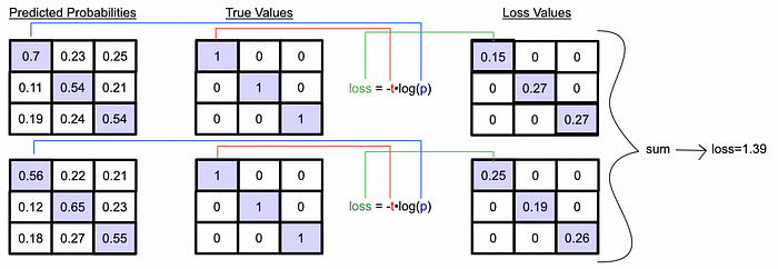
Going from probabilities via the two softmax approaches to a single loss value The astute among you might realize a peculiar incompatibility here. The whole point of contrastive learning is that you’re learning to optimize both positive and negative pairs. We want to push positive pairs close together, while pushing negative pairs apart. How can we learn to push negative pairs apart if their loss (the thing we’re optimizing) is zero no matter what we do? (negative pairs are identified as having a true value of zero, which sets the log loss of negative pairs to always be zero)
This is a sneaky but incredibly important characteristic of the softmax function: when the probability of negative pairs get bigger, the probability of positive pairs get smaller as a direct consequence. As a result, by optimizing for positive pairs to be as close to 1 as possible, we’re also optimizing for the cosine distance between negative pairs to be as small as possible.
Using CLIP
I touched on these use cases of CLIP previously, but I wanted to reiterate now that we have a more thorough understanding of CLIP.
Use 1: Image Classifier
Given an input image, we can pass a variety of textual descriptions to CLIP and calculate which description best represents the image. We can do this by passing the image through the image encoder, all text through the text encoder, and calculate the cosine similarity between the image and all text inputs via a dot product of their embedding. We can then compute the softmax across all similarity values to compute a probability that a piece of text belongs to an image.
Use 2: Image Search
Similarly to building an image classifier, we can pass some phrase into the text encoder, multiple images to the image encoder, compute the dot product and softmax, and thus get a probability of which image is most relevant to a piece of text.
Use 3: Image Encoder
Because CLIP is good at representing the content of images generally, we can use the image encoder for downstream tasks. I cover an example of this here.
Use 4: Text Encoder
Because CLIP is good at representing understanding which aspects of a linguistic phrase are relevant to images, we can use the text encoder for downstream tasks.
Conclusion
And that’s it! Good job for sticking in there. CLIP is fascinating and incredibly powerful, but because it’s so fundamentally different than more straightforward approaches it can be difficult to wrap your head around.
In this post we covered the high level reasons of why CLIP exists and what it generally does. Then we broke CLIP down into three components; the image encoder, the text encoder, and the jointly aligned embedding space used to bridge the two together. We went over the high level intuition of how CLIP uses large batches to create numerous positive and negative pairs, then we drilled down into the loss function used to optimize CLIP.
'Research > Multimodal' 카테고리의 다른 글
SimCLR (0) 2024.09.26 Learned latent queries 의 정체 (0) 2024.09.26 Visual Question Answering with Frozen Large Language Models (0) 2024.09.25 Perceiver 과 Flamingo에서의 Perceiver Resampler의 미묘한 차이 (0) 2024.09.24 [Flamingo] The architecture behind modern visual language modeling (0) 2024.09.24