Rejection Sampling

※ https://towardsdatascience.com/what-is-rejection-sampling-1f6aff92330d

---

Rejection sampling is a Monte Carlo algorithm to sample data from a sophisticated ("difficult to sample from") distribution with the help of a proxy distribution.

 

What is Monte Carlo?

 

If a method/algorithm uses random numbers to slove a problem it is classified as a Monte Carlo method. In the context of Rejection sampling, Monte Carlo (aka randomness) assists in implementing a criterion in the algorithm.

---

Terminology & Notations

• Target (distribution) function f(x) - The "difficult to sample from" distribution. Our distribution of interest!
• Proposal (distribution) function g(x) - The proxy distribution from which we can sample.

---

The Big Idea

With respect to sampling, the central idea that is present in almost all Monte Carlo methods is that if you can not sample from your target distribution function then use another distribution function (and hence called as proposal function).

 

However, a sampling procedure must "follow the target distribution". Following a "target distribution" implies that we should end up with several samples per their likelihood of occurrence. In simple words, there should be more samples from regions of high probability.

 

This also means that when we use a proposal function we must introduce the necessary corrections to make sure that our sampling procedure is following the target distribution function! This "corrective" aspect then takes the form of an acceptance criterion.

---

How does it work?

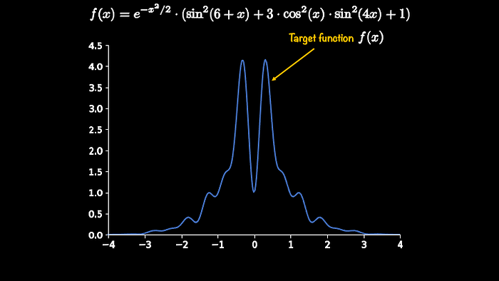
I will explain the algorithm with the help of an example. Consider a target distribution function from which we can not sample. The plot and its functional form are shown below.

 

This is a one-dimensional target function and our task is get samples that fall in between -3 and 3. One choice of proposal function is ts the uniform distribution function. Below is shown its functional form i.e. g(x).

 

If I take this proposal function and plot it alongside our target function then it would look like this:

 

As you can see that at present our proposal function does not completely encapsulate our target function. The significance of this encapsulation will get clear once we will formulate the corrective measure (or acceptance criterion).

 

One simple remedy is to scale the proposal function but then what should be that scaling constant? ... This is one challenge with rejection sampling but for a simpler one-dimensional target function, you can get it by maximization. This scaling constant is indicated using a symbol C or M. 

 

After scaling, our plot will look like this. The value of C is 25 for this example.

 

Now we are ready to sample using our proposal function. We will then evaluate both these functions for the samples.

 

The sample is marked using the orange X. The  pink point shows its value for f(x). You can also see where it will evaluate for the proposal function g(x). As such since we have used uniform distribution as a proposal function all the samples are equally likely and they will all evaluate to C g(x).

 

Now we need to come with a criterion that will help in making sure that we will end up following the target distribution function. The above plot should help us form an initial intuition about this criterion. I am going to call the vertical line on which you see the pink point and orange X, the evaluation line.

 

You should think in this direction - "If somehow I can get a number on this evaluation line and if this number falls below the pink point then I will accept the sample X else I will reject it”.

 

But from where this so-called number will come from and how can we ensure that it will fall on this so-called evaluation line?

 

This is where we make use of randomness (aka Monte Carlo notion). But before that let me show you a rotated version of this plot that presents a better visualization (and hopefully leading to a better intuition).

 

In this rotated version, we can see that we have an axis whose range is (0, Cg(x)), and our criterion to accept X would be to use another number that falls between 0 and Cg(x). If this number is on the left of the pink point we accept our sample else we reject it.

 

The big idea here is that the portions of the line on the left and right of the pink marker are not equal and also (somewhere) reflect the chances of occurrence of the sample. But the question remains who will give us this number that will fall on this evaluation line?

 

To get this number we will use another uniform distribution with limits from 0 to Cg(x). Even though all the random numbers from uniform distribution are equally likely we can see that there will be more numbers falling on the right side of our evaluation line as it is bigger in size. This usage of randomness is what gets this algorithm classified as a Monte Carlo algorithm. Here are two plots that show the acceptance and rejection events.

 

Based on the above explanation you can see that our acceptance criterion for X can be represented mathematically as:

 

which is the same as saying that if "u" falls below the pink point then we accept!... see the below plot in its original form:

 

It is important to note that when the sample is rejected we discard it and repeat the process i.e.

• get another sample from the proposal function
• get a random number (u) between 0 & Cg(x) from a uniform distribution function
• check if u ≤ f(x); if true accept it else reject it
• repeat

I also want you to get familiar with another formulation of this acceptance criterion. In this formulation, we will get “u” from a uniform distribution that gives us the samples from 0 to 1 i.e. the standard uniform distribution. If you use that then the acceptance criterion will look like as shown below:

 

If we repeat this algorithm many times we would end up having a plot that would look like this:

 

As should be evident, a lot of samples will be rejected 😩

 

One remedy is to reduce the rejection area by choosing another proposal distribution function. Remember that you would choose the proposal distribution function from which you can sample as well as it can encapsulate the target function (after scaling of course!). Below I am showing you the usage of Gaussian distribution as a proposal function.

 

The rejection region has now significantly reduced. The scaling constant C is 11 in this case.

---

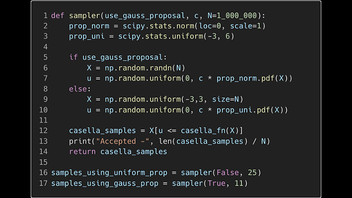
A simple python implementation

 

Using the above simple python implementation, I tried both of our proposal distribution functions (i.e. uniform and gaussian), and here are the results:

 

As expected, the choice of Gaussian distribution as a proposal function is much better (53.63% acceptance rate) but still quite inefficient!

---

Limitations & Challenges with Rejection Sampling

• Selecting the appropriate proposal function & finding its scaling constant
• Requires that the PDF of the target function is known
• Generally inefficient especially in higher dimensions