[Lecture 7] (1/2) Function Approximation

https://storage.googleapis.com/deepmind-media/UCL%20x%20DeepMind%202021/Lecture%207-%20Function%20approximation%20in%20reinforcement%20learning%20.pdf

https://www.youtube.com/watch?v=ook46h2Jfb4&list=PLqYmG7hTraZDVH599EItlEWsUOsJbAodm&index=7

---

---

The policy, value function, model, and agent state update, all of these things that are inside the agent can be viewed as being functions. For instance, a policy maps the agent's state to an action or to a stochastic policy from which you can sample an action. A value function maps a state to a value which is an estimate of the cumulative reward into the future. The agent state update itself maps the previous agent state and the observation into some new agent state.

---

---

We have in mind when we think about reinforcement learning, we want algorithms that can be applied to the setting where the environment is just humongously large and the agent must be necessarily a lot smaller. So the mind of the agent including its memory capacity must be necessarily smaller than the environment. 

---

A different problem is also too slow to learn the value of each state individually. So think of it this way so if you have a problem that is not too large, let's say there's a million different states, we can store a million numbers in modern computers that's not a problem at all but then still if you would update each of these state values individually and separately then it would take quite a bit of experience to learn reasonable value estimates for each of these states. And indeed this feels inefficient. 

 

If these states have some commonalities which we would then completely be ignoring so if these states can instead be viewed as being similar to each other then maybe you would want the value of a certain state to be updated when the value of very similar state is updated. This is called generalization.

 

So our solution for all of these problems will be to introduce function approximation.

---

We're going to introduct some parameter vector w where the value function is parameterized with this w. It's a functional state somehow where the state is the agent state and we're either approximating the value of a certain policy or the optimal value function. 

 

We're going to approximate these and then update the parameter using Monte Carlo algorithms or TD learning. And then hopefully if we pick our function class correctly, we will be able to generalize to unseen states. 

 

So in any case if you have such a function, the values of these unseen states will be well-defined. 

---

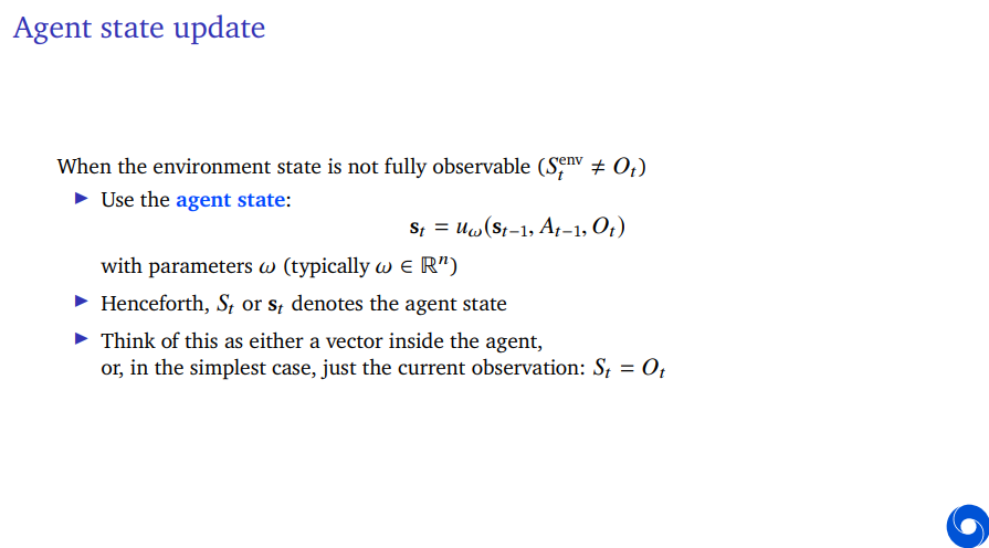
One of the problems might be that the environment is not fully observable. So the environment state is not equal to the observation then as always we're going to rely on the agent state instead. 

 

And we could also consider the agent state update function to be a parametric function of its inputs which are the previous agent states, the action and the observation and potentially the reward as well if that's not part of the observation, and it has some parameters omega.

 

This agent states should contain everything that's useful for you to make value predictions or to pick your policy and that means that the agent update function is quite important and might need to capture things like memory. It might be that you have to remember what you've seen before. 

---

The tabular case, where we have a table. So our function class here is tabular. And then one step up from that would be state aggregation. So in a table, we have an entry for every single state for instance let's consider for simplicity that is fully observable, so you observe the environment state and you just have an entry for every environment state. In state aggregation, you would instead have an entry that merges the values of a couple of states. So we just partition the state space into some discrete small set potentially so that we can maybe learn the values of these partitions instead of learning them for every individual state. And then we would get some generalization. Because all of the states in the same partition would then be updated with the same algorithm and hence would obtain the same value. So if you reach a new state in a certain partition that you haven't seen before, then it would automatically already have a value and it might be a suitable pattern.

 

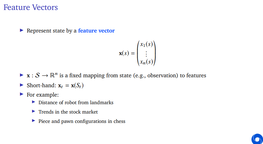
Now one step up from this will be linear function approximation. And now consider a fixed agent state update function and a fixed feature map. So this is why things will be linear because we're going to assume that the agent state update function doesn't have any parameters, the feature map doesn't have any parameters and instead all that we're going to learn are the parameters of the value function which uses those features as input. 

 

State aggregation and tabular are special cases of linear FA. (one-hot representation)

 

Now one step up from that, if we're going to be even more flexible would be to consider differentiable function approximation. In this case, our value function will be a differentiable function of parameters w. And it could be non-linear. 

 

One way to interpret this is that, you can consider the feature mapping now no longer to be fixed. So we take whatever the agent state as input and for instance, the input could just be the observations, could be the pixels on the screen when we're playing an Atari game or something like that and then instead of having a fixed feature mapping, you could consider this to be a learned feature mapping where something maps it into features. And then there's an additional parameter on top of that, that maps it into values.

 

Why we call this differentiable function approximation is that, we can still compute gradients because we're going to consider gradient-based algorithms. And it allows for veery rich function classes such as deep neural networks.

---

Agent's policy affects the data it receives. What I mean with this is that, the reinforcement is an active problem and this has multiple consequences including that actually one benefit of this is that, you can actively sample data in a way that is useful for learning your function. You could literally have an exploration technique that maybe seeks out certain parts of the state space in order to improve your value estimate specifically over there. 

 

It also causes some issues for instance, the regression targets are often non-stationary. This is because we're doing control like we might be changing our policies as we go and this might not just change the targets for our regression, our value targets for instance if we bootstrap. But it might also change the data. So it's non-stationary in more than one way. 

 

Even if the policy is fixed, the targets might change because your value estimates that you're using to construct your targets could be changing. So in TD, we're using our value estimates and those initially are not very good but later they might become more accurate.

---

The tabular case, we have really good theory, we understand these algorithms really well. We know when they converge, we know where they converge, they're quite stable. The assumptions for convergence are not very strict. So you can fairly easily apply them and be pretty certain that they will learn something. And they also tend to learn relatively well and fast if the state space is small enough. But they don't generalize. They don't scale. You can't apply them to very large problems. 

 

In the linear case, we're already a little bit more flexible on our function class. We still have reasonable boost theory, so we understand these methods quite well. We know when they converge and where they converge in many cases. But we are dependent on this fixed feature mapping. So we do require very good features. 

 

And there's non-linear function approximation which is less well understood. But it scales really well and it tends to work quite well in practice until it doesn't. And then sometimes we don't really understand what's going on in some edge cases. But our experience with this and our understanding of this has been growing quite a lot over the recent years. And it's really flexible.

 

And importantly, it's much less reliant on picking good features by hand. One thing that this means is that you can apply these methods to problems that you don't really understand that well, but as long as you have a well formulated reward function that you are certain is the right reward function, you could apply these reinforcement methods and then still get better find good policies for these domains without really needing to understand what appropriate features would be.

 

And in fact we see more often these days over and over not just in reinforcement learning but also in deep learning and related fields when applied these algorithms that don't try to hand engineer feature but instead try to learn them from data, tend to outperform methods in which these features are hand engineered. 

---

---

J is a number that depends on your parameters w and the way it depends on that here, we define it to be the expectation over some distribution of states due to your policy and the MDP dynamics and we want to consider the square difference between the actual value of your policy and our current estimate. That's something that we might want to minimize. This will be a predictive loss. 

 

Update to the weights, delta w would be small step size alpha times the expectation under that distribution over states of the target which is our true value function for that state minus our current prediction times the gradient of that current prediction. 

 

This is an expectation so we can't typically use that until unless we really have the distribution over states but if we want to use this in practice, we can sample this. 

 

That means that we're going to sample the state we're in and we're also going to sample this true value of the policy and one way to do that would be to plug in the Monte Carlo return which is an unbiased estimate for the true value of the policy. 

 

So this stochastic gradient descent update is an unbiased estimate of the gradient descent algorithm. 

 

And that means if we take our step size to be small enough and we take enough of these steps, we will on average move in the direction of the gradients and we will reach the same solutions as the great as the full gradient algorithm would. 

 

And it's another reason to pick a small step size so not just because then the gradient is valid but now also to average out the noise in our estimate of the gradient. 

---

---

We're going to subdivide this space but into overlapping regions and then whenever we're in such a region, so we're here at this x say, and then we're going to have a feature that is associated with each of these circles when you're in the circle the feature will be one and whenever you're outside of the circle, it might be zero.

 

If you do that with this representation, in this case three features will be equal to one and all the other features would be equal to zero. So this is no longer a one-hot representation as for the state aggregation or the tabular cases.

 

In this case it would be a few-shot representation. In some sense the features are still binary, either zero or one, but it's some sense already a richer representation because if you get these three regions in some sense to light up we actually know we must be in the intersection of all three of them and that can be useful information but in addition to that we still have some generalization. 

 

If we're going to update the value associated with a state in this very darkest region over here, that means that a different state say at y will also be updated a little bit because it shares one of the features with this state that is going to be updated. 

 

So if we think of the linear function that is going to be applied to this. It'll have a weight associated with each of the features, so if we change the weight of that feature that means that any position that shares that feature where that feature is one will also experience a slight change in its value.

 

Now I described the binary case for simplicity where you're either in a region or you're out and your associated feature either one or zero, but that's not the only option. You have some sort of a distance function that might be Gaussian and instead of you're in a circle or you're out, we have a bunch of center points of these circles and we just measure how far you are from each and every one of them.

 

The idea is then you have your representation and you expand this into a whole bunch of different features and then you can press that with your weights.

 

Why do we expand? This case note that we had a two-dimensional representation. We could have had an x-y location which would constitute two numbers and we could have fed thta to the agent. But it's really hard for the agents to turn those two numbers with a linear function into a valid value estimate. The only thing you can do then is some sort of a linear function over the state space. You can't have any non-linearity in terms of your location and how the value reacts to your location if you would only feed in the actual location numbers, the x, y coordinates.

 

So what we're doing instead is, we're turing those two numbers of this two-dimensional space into very many numbers as many as we've defined these circles. So in some sense we're actually blowing up the representation in order to then be able to apply a linear function to that. This is a common technique. 

 

We're blowing up the feature space into something large in the hope that then the feature representation will be rich enough that a linear function suffices that if you then apply a linear function to these features, you still have a good enough approximation. 

 

There are some limitations to this approach. It might be hard to figure out a good subdivision of that space without making the feature representations extremely large. This is sometimes called the curse of dimensionality. 

---

There is a choice. Narrow generalization, we've picked these circles to be fairly small and what this does is, it allows you to be quite specific so if the value function is updated, only in this region that lights up and then maybe mostly updated in the smallest region because of your representation that means that you have narrower generalization. 

 

If you update this state, states fairly near to it get updates as well, but states further along or not. And that's both good and bad, this is a double edged sword if you have narrower generalization, this means the narrower it becomes, the more specific your value function can be and the more precise it can be if you need veery like high resolution in some sense in your value function because the actual value function might for instance be quite bumpy or weird then it might be useful to have very narrow generalization. 

 

But it does mean that learning might progress quite slowly because there's very little leaking from the state information from states further away.

 

So instead you could consider having broad generalization where the overlap is much larger the circles are much larger, then updating just a state in the middle would actually update a fairly large region of your state space and this can be useful because it might speed up learning. But you lose out in terms of your resolution at the limit when you've learned your value function. There's a limit to how precise you can make it at every situation depending on your dimensions .

 

It could be that you want to pick something more custom that the best representation would be asymmetric. This shows it alludes to the fact that it can be quite tricky to pick these things in general. 

---