-
[Lecture 5] Model-Free PredictionResearch/RL_DeepMind 2024. 7. 30. 15:54
https://www.youtube.com/watch?v=eaWfWoVUTEw&list=PLqYmG7hTraZDVH599EItlEWsUOsJbAodm&index=5


In general, in reinforcement learning when people say Monte Carlo, they typically mean sample complete episodes, an episode is a trajectory of experience which has some sort of a natural ending point beyond which you're not trying to predict any further.
This is a model-free approach, because you don't need any knowledge of the Markov Decision Process. You only need interaction or samples.

The true action value is given on the RHS. which is the expected reward given an action, and then the estimates at some time step t is the average of the rewards given that you've taken that action on the sebsequent time steps.
And we can also update this incrementally where you have some step size parameter alpha and, you add to the action value estimate that you have right now (qt(At)), and you add the step size parameter times an error term.
This error term is the reward that you've just observed minus our current estimate.
All the other action values stay unchanged.
And then if you pick this step size parameter to be exactly one over the number of times you've selected that action, then this is exactly equivalent to the flat average that is depicted above.

The goal is to estimate the expected reward conditioned not just on action but also on the state.
These are called contextual bandits where the state is often called a context. So state and context in that sense are interchangeable terms.


So our solution for those problems is to use function approximation.
We write v_w or q_w where w is now some sort of a parameter vector and we're going to update these parameters instead of updating cells in a big table. So the parameter vector w will be updated using Monte Carlo or Temporal Difference learning.
The idea would be that we can hopefully then generalize to unseen states because this function should be defined everywhere and the idea is that if you pick a suitable function, then if you update a certain state value in some sense you update your parameters that are associated to that state, then the values of similar states would also automatically be updated.
For instance, you would be in this state, you could identify that state by looking at certain characteristics, certain features and then you could update the values of those features and then maybe if you reach a different state which is different in some ways but it shares a couple of those features maybe we can make a meaningful generalization and learn something about its value before even visiting it.

Agent state update function: subsequent agent states St is a function of these previous inputs.


x_t: features of state at time step t.
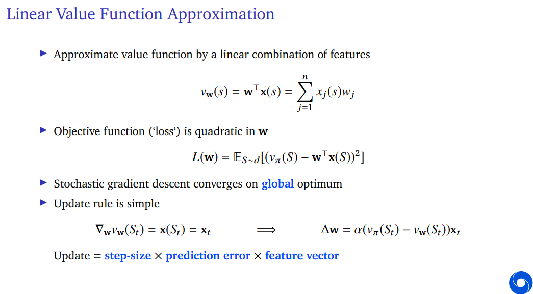
The linear function approximation approach takes these features and simply defines our value function to be the inner product or dot product between our parameter vector w and the features at the time step x(s).


Gradient update: stepsize times an error term (reward minus our current estimate) times the gradient of this action value.
And then, we can sample this to get a stochastic gradient update.
It will converge to the right estimates where these estimates are limited in the sense that you can't expect all of your values to be perfect because it might be that your function class is just not rich enough to get all the values completely accurate in every state, but this process will converge under suitable assumptions to the best parameter vector that you can find.


We have to wait until an episode ends before we can learn. We're using the full return of an episode to update towards and that means we have to wait until the episode ends before we even have the thing that we want to use in our update.
In addition these returns can have very high variance in some cases especially if episodes are long.


The Bellman equation relates the value of a state with the value of the next state or the expected value of the next state. This is a definition of the value of a policy.
The value of a policy is defined as the expected return, but turns out to be equivalent to the expected immediate reward (R_t+1) plus the discounted true value of that policy in the next state (S_t+1).
We can approximate these values by iterating basically turning the definition of the value into an update. So the difference here is now that the v_pi within the expectation has been replaced with our current estimates v_k, because we're doing this in iterations maybe across all states at the same time.
So we denote this with this iteration with some number k and then we update our value function by replacing maybe all of them at the same time. You could do this for all states at the same time with a new estimate v_k+1, which is defined as the immediate reward R_t+1 plus the discounted current estimate of the next state value v_k.
We've seen that these algorithms actually do learn and they do find the true value of policy.
Now there's on the RHS an expectation, we could sample that. So we can just plug that in. We just see sampled R_t+1 plus the discounted value of the next state S_t+1 and then use that.
That's going to be too noisy, so instead just take a small step.
This looks similar to the Monte Carlo learning algorithm, but instead of updating towards a full return, we're going to update towards this other target which is the reward plus the discounted estimate for the next state.
So the change here between Monte Carlo learning and this algorithm is that, we've replace the full return with something that uses our current value estimates.

This is called Temporal difference learning because, the error term here is called a temporal difference error which looks at one step into the future and looks at the difference in value from what we currently think and comparing that to one step into the future.
This temporal differnce error which is simply defined as R_t+1 plus the discounted value of this state S_t+1 minus our current value estimate of the value at S_t is called the temporal difference error and we typically denote this with a delta t.

Dynamic Programming works like this. There's some tree of possibilities here. You're in some states and you consider all the possible possibilities that that might happen next.
States here are denoted by white nodes, actions are black nodes.
The dynamic programming looks at all possible actions, in this case two, and then also at all possible transitions for each action. So in this case each action can then randomly end up in two different states so there's four states in total that you could end up in after one step.
Dynamic programming considers all of these which requires you to have a model that allows you to consider all of these possibilities.

Conversely, Monte-Carlo learning takes a trajectory that samples an episode all the way until the end. This terminal state denoted with a green box.
And then it uses that trajectory to construct the return and updates the value of that state at the beginning towards that return.
And you could also update all of the other states along the way towards the return from thta state.

Temporal difference learning instead only uses one sample.
So we see some commonalities with dynamic programming in the sense that we're only doing one step, but but it does sample, so it doesn't need a model. So there's some commonality with dynamic programming in the sense, we're only doing one step deep and there's some commonality with Monte Carlo learning in the sense that we're sampling.

※ Statistic에서 말하는 Bootstrapping과 의미가 다름 주의!
* Bootstrapping in RL: usage of our estimates on the next time step. Process of using a value estimate to update your value estimate.
* Bootstrapping in statistic: taking a data set and then resampling from the data set as if it's the underlying distribution.
Monte Carlo learning does not bootstrap. It does not use value estimates to bootstrap upon to construct its return, its targets. But dynamic programming does and temporal difference learning also does these both use our current value estimates as part of the target for their update.
And then, the Monte Carlo samples but dynamic programming does not sample. It instead uses the model and temporal difference learning does sample.


If the episode is really long, you don't have to wait until all of the way in the end of the episode before you can start learning. This can be quite beneficial because then you can also learn during the episode.

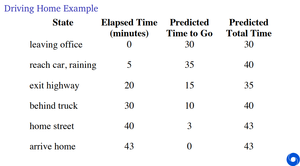

The Monte Carlo algorithm would just look at the total outcome and therefore it would then update all of these states that you've seen so far to take into accout this new total outcome.
In Temporal Difference learning, we're thinking when we've reached our car, actually it's more like 40 minutes in total, so we should update that previous state value upwards to 40. And you can immediately excute that. You could immediately update that state value.


The computation of Temporal Difference learning is constant on every time step. How many steps you want to do in an episode does not matter in terms of the computational complexity on each time step for Temporal Difference learning.
So why is that not true for Monte Carlo? Monte Carlo needs to store everything. So TD can learn from single transition but Monte Carlo must store all the predictions you've seen in an episode in order to able to update them at the end of the episode. So that means that the memory requirements for Monte Carlo grow when the episode becomes longer and longer.
But Temporal Difference learning needs reasonable value estimates. If these value estimates are very bad, then obviously if you're going to construct targets using these, then maybe your updates won't be very good.


The world may be partially observable. The states that we're plugging into these value estimates might not tell us everything.


We know that tabular Monte Carlo and Temporal Difference learing do converge to the true value estimates. So if we store all the values separately in the table, we can update all of them independently to eventually become accurate under the conditions that your experience goes to infinity and your step size decays slowly towards zero.
But what about finite experience in practice?
So what we're going to do is, we're going to consider a fixed batch of experience and specifically we're going to consider having collected k different episodes and each of these episodes will consist of a number of steps.
So these number of steps per episodes can differ but they might all have a large or small number of steps. And then we're going to repeat each sample from these episodes and apply either MC or TD.
You can view this as sampling from an empirical model where we talked about in the dynamic programming having a model and then being able to use that to learn, in this case, you could also consider having the data set which in some sense defines observed frequencies of transitions which is similar to having a model but it's an empirical model and it won't exactly fit with the real underlying model because you only have a finite amount of experience.

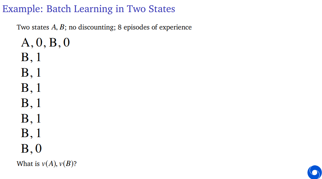


MC converges to the best mean squared fit for the observed returns. We sum over the k episodes from 1 to K and then within each eposode, we look at all the time steps from 1 to T_k for that eposode. And then we could look at all of the returns that you've seen and compare that to our current value estimates and then we could say, we want to minimize the squared error between these returns that we've observed and these value estimates.
We're minimizing the difference between the returns we have seen and the value estimates that we have.
TD converges to the solution of the max likelihood Markov model, given the data. That's what we saw on the previous slide. This is the most likely model given the data that we've seen so far. And then TD learning turns out finds that solution that corresponds to this model.
So this would be the solution of the empirical Markov Decision Process assuming that the empirical data you've seen is actually the true data.


Now maybe a natural question is, can we maybe get the best of both?
We put dynamic programming in the top left and the reason why it's there is that, left corresponds to shallow updates where we just look one step into the future.
The top versus bottom, in the top, we look at mechanisms that look full breath. Of course, in order to do that, you do need to have access to the model. So that means that, for instance, if we look both full breadth and full depth, this would give you exhaustive search.
If we go down, we go to these algorithms that only look at one trajectory and these can be used when we only can sample.
So we see Temporal Difference learning in the bottom left and Monte Carlo in the bottom right where we can think now about Temporal Difference learning as having a breadth of one but also only a depth of one. So we can just take one step in the world and we can use that to update a value estimate. Whereas Monte Carlo makes a very deep update. It rolls forward all the way until the end of the episode and uses that full trajectory. Then update its value estimates.

TD, information can propagate back quite slowly. This means that if we see a reward that is quite useful like, it's a surprising reward, Temporal Difference learning will by it's nature, only update the state value immediately in front of it, if in that episode you never reach that state again, that means that all of the other state values don't learn this reward. Whereas Monte Carlo would update all of the previous states that you visited in that episode eventually to learn about this new reward. So that means that Temporal Difference learning has a problem in the sense that information can propagate quite slowly backwards and therefore the credit assignment could be quite slow.

We can actually go in between these. One way to do that is, instead of looking exactly one step ahead as Temporal Difference learning does, we could consider looking two steps ahead or three steps or generically n steps ahead.
Then we could consider Monte Carlo learning to be at the other end of other extreme where Monte Carlo looks infinitely far into the future up until the end of the episode.

In between, we could consider, for instance a two-step approach which takes not just one reward but takes two rewards into account then bootstraps on the value of the state time step t+2.
And then we can use this in our updates. So does that mean that we have to wait a little bit of time before we can execute this update and we do have to store some estimates or states along the way but only as many as we want.


SARSA is TD for action values. If we look on the left, we see a specific path that was taken. We started over here then we went right, right, up, right, up and so on in the end, we reached the goal. If we would then do one step TD, in this case, one step SARSA, we would only update the state action value for the action that led immediately to the goal. This is assuming that all of the other intermediate steps have no information.
If we could then instead consider a 10-step update, it would update all of these state values appropriately discounted along the way. So it would propagate the information much further back. And then if we consider the next episode, this could be beneficial.
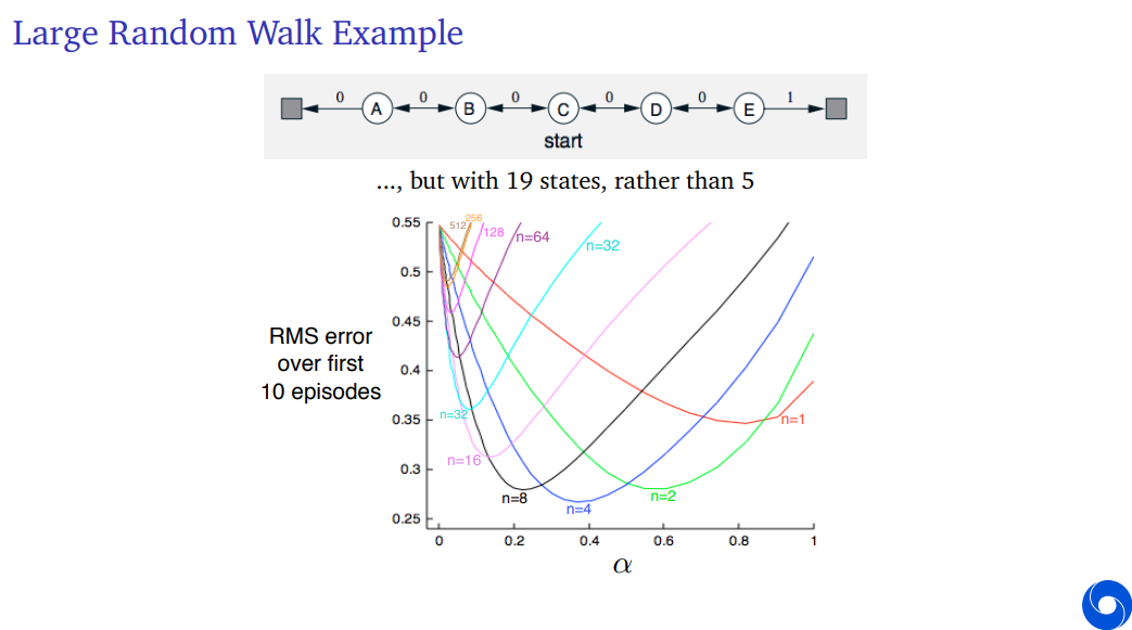
We can apply this to a Random Walk. We can apply these n-step algorithm, and see how they fare. So what you see here is something called a parameter plot because on the x-axis, we have a parameter in this case the step size parameter, and on the y-axis, we see the root mean squared error over the first 10 episodes.
So we're not looking at infinite experience, we're just looking at a finite amount of experience and then we see how do these algorithms fare.
If you look at all of these different step sizes, let's look at n is one. One corresponds exactly to the normal Temporal Difference learning algorithm. We see that the best performance or the lowest error if we only care about the first 10 episodes and we have to pick a constant step size 0.8, if you set it higher or lower, the error is a little bit worse.
If we consider a two-step approach, we see that if the step size is really high, if it's one, than it actually does a little bit worse. This is because the variance is in some sense higher but you can tune your step size around 0.6 to get lower errors than where possible with the one step approach.
Then taking n is 4 is maybe even a little bit better but notice again that the preferred step size parameter is again a little bit lower.
This is because, if we increase n, the variance goes up more and more and that implies that we need a lower step size to make sure that we don't have updates that have too high variance which would make our error higher.
Then if we go all the way up, we see a line that is marked with the number 512, that is a 512 step Temporal Difference learning algorithm which in this case is essentially Monter Carlo, because the probability of having an episode that is more than 512 steps long is very small.
We can also see that by the fact that the 256 step Temporal Difference learning algorithm is actually quite similar because both of those are already quite similar to the full Monte Carlo algorithm.
For these algorithms, we see two things. First, they prefer veery small step sizes of much smaller than Temporal Difference learning. In addition, even if you tune the constant step size very well, the error will still quite high.
So we clearly see a bias-variance trade-off. Intermediate value of n helps us learn faster and helps us get lower error over the first 10 episodes for a well-tuned step size parameter and the best values are not the extremes. So it's not n is one and it's also not n is infinity. So it's not TD, it's not MC. But it's some intermediate n-step TD algorithm.


On some of these steps, we fully continue with the random sample with the trajectory, whereas on other steps we fully stop we just say okay that's enough, bootstrap here. You could bootstrap a little bit.
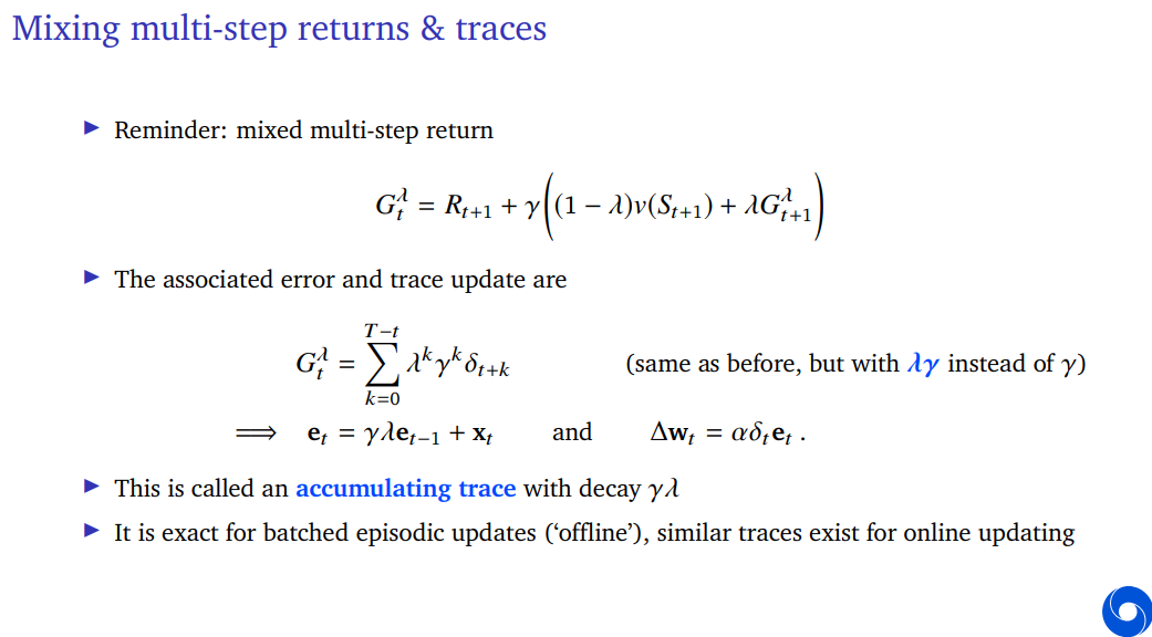
You could have a parameter lambda, so we're going to take one step as always and then we're going to take the discount factor but then instead of either continuing or bootstrapping fully, we say, let's bootstrap a little bit. So this is a linear interpolation between our estimated state value and the rest of that lambda return.


Multi-step approaches are not independent of span which means that, similar to Monte Carlo, you have to wait all the way until the end of the episode before you know your lambda return. The lambda that trades off statistical properties of the updates but it still has the same computational update that you can only construct your full lambda return when you've reaches the end of the episode.
Now that doesn't seem very desirable and indeed you might also sometimes want to do Monte Carlo learning and then that might also not be desirable. Conversely, temporal difference learning can update immediately and is independent of the span of the predictions.
So before you took this to be an argument that we should be using temporal difference learning, but here I'm going to make a different argument and we're going to ask can we get the best of both worlds? can we use these mixed multi-step returns or like other flavors of that including even Monte Carlo but with an algorithm that doesn't have computational requirements that grow indefinitely during the episode?
I'm going to explain to you how that works.

We have a value function that is a linear function. So we have a value function defined as an inner product of a weight vector w with some features x. And then Monte Carlo and Temporal Difference learning, the update to the weights can be written as follows.
For Monte Carlo learning, it's a step size times your return minus current estimates times features. And for Temporal Difference learning, is your step size times your temporal difference error times your features.
And then for Monte Carlo learning, we can update all states in an episode at once. So this is typical, because you have to wait for the end of the episode for all states anyway to know the return. So it's quite typical for Monte Carlo learning to then just update all of them at once in one big batch.
Here, we're going to use t from 0 to T-1 to enumerate all of the time steps in this specific episode.

Now, I'm going to argue that, we can look at these individual updates, here we have an update on every time step and we just summation over time steps. (previous slide) I'm going to argue that you can define an update as follows.
This update is a very simple update that takes an alpha, step size parameter, times, your one step TD error, this is not your Monte Carlo return, this is the one step TD error, times, some vector e.
This e is called an eligibility trace and it's defined recursively by taking the previous trace, decaying it according to gamma and lambda and then adding our current feature vector, more generally your gradient x_t.
Note, special case, if lambda is zero, we get one-step TD.
So there's choice here, whether you want to do online TD which means you update during the episode, you could also consider offline TD where you still just accumultate these weight updates until the end of the episode.
The intuition is, we're storing a vector that calls all of the eligibilities of past states for the current temporal difference error and then we're going to add that to our update to the weights. So when lambda is not zero, we have this kind of trace that goes into the past, similar to momentum, but it serves a slightly different purpose here, which will hold recursively this e_t-1 will therefore hold the x_t-1, the features from the previous state, but properly decayed. And also x_t-2 and so on and so on, each decaded even more.
So this is kind of magical, I haven't yet shown you why it works or how it works but this means that if this works, we can update all of the past states to account for the new temporal difference error with a single update. We don't need to re-compute their values. We don't need to store them. So this would be an algorithm if it works that will be independent of the temporal span of the predictions. We don't need to store all of the individual features x_t, x_t-1, x_t-2 and so on and so on. Instead, we just merge them together by adding them into this vector and we only have to store that vector.

How does that look? There's a Markov Decision Process here, in which we only ever step down or right in the end we reach some goal states from which we get a reward of +1 and this then we transition all the way back to the top. So the trajectory will be somewhat random. The true values are larget the closer, we are to that goal.
If we then imagine doing only one episode, TD(0) would only update the last state, so the state in which we saw that one reward. TD(lambda) would instead update all of the state values along the way less and less.
So with lambda, this is true if you do the version that we had before with the lambda return, but turns out the exact same thing is also true if you use these eligibility traces.
And the way to think about that is, that at some point, we see this temporal difference error where we finally see this reward of +1 that we've never seen before and then we multiply that in with all of these taking into account all of these previous features that we've seen. In this case, it's tabular, so all of the features are one hot but so we're storing all of the states in this vector and we're updating it in one go.

We notice that we can write the total Monte Carlo error as a sum of one step Temporal Difference error.

Now we're going to go back to this total update. So at the end of the episode, we're going to update all of our weights according to all of these Monte Carlo returns that we've seen constructed so far which we've only were able to construct at the end of the episode. Now I'm going to plug in this thing that we derived in the previous slide, where we're replacing this Monte Carlo error with this summation over time of temporal difference errors.
Note that the summation only starts at time step t which is the time step from which the Monte Carlo return also starts.
This rest thing that we have here, it's a discounted sum of feature vectors and we call that e.
Originally, we had for every state, we had this update of a return looking into the future. This is why we had to wait all the way until the end of the episode because we have to wait for Gt to be completely defined.
And we swap this around to a summation where we have our same step size and our temporal difference error delta t and then this weight vector which looks into the past. It stores all of the feature vectors that we've seen in previous states.

So our total update can be written as this where this eligibility trace vector was defined as the summation up to time step t of our discounted feature vectors.

We have this immediate update for every time step, we have all these quantities available for us at time step t, then the Monte Carlo update would sum all of these deltas over all of the time steps in the episode, and then apply them.
This is the off-line algorithm. So in this case, even though we can compute these things along the way, we can now compute this sum incrementally as we go. So we don't have growing memory requirements. But then, in this specific algorithm, we're still applying them at the end. Can't we just apply them during the episode? and yes, indded you can so. You can now start doing something that would be equivalent to Monte Carlo if you would wait all the way until the end of the episode and only then apply these differences but you could already start learning journey durning the episode.
So we haven't just reached an algorithm that has the property that is independent of span which is a computational property, but we've also arrived at an algorithm which is now able to update it's predictions during logn episodes, even though we started with the Monte Carlo algorithm.


The intuition of this update is that, the same temporal difference error shows up in multiple Monte Carlo erros. In fact, in all of the Monte Carlo errors for states that happened before this time step. And then what we do is, we group all of these states together and apply this in one update. You can't always do that but you can to that here.

'Research > RL_DeepMind' 카테고리의 다른 글
[Lecture 6] (2/2) Model-Free Control (0) 2024.08.02 [Lecture 6] (1/2) Model-Free Control (0) 2024.07.31 [Lecture 4] Theoretical Fundamentals of Dynamic Programming (0) 2024.07.30 [Lecture 3] Markov Decision Processes and Dynamic Programming (0) 2024.07.29 [Lecture 2] Exploration and Exploitation (0) 2024.07.29