code example (4): Randomization Inference

https://mixtape.scunning.com/04-potential_outcomes#methodology-of-fishers-sharp-null

---

Fisher's sharp null & Steps to a p-value

You can never let the fundamental problem of causal inference get away from you: we never know a causal effect. We only estimate it. And then we rely on other procedures to give us reasons to believe the number we calculated is probably a causal effect. Randomization inference, like all inference, is epistemological scaffolding for a particular kind of belief — specifically, the likelihood that chance created this observed value through a particular kind of procedure.

randomization inference procedure will become a more interesting and powerful tool for making credible causal statements.

The main advantage of randomization inference is that it allows us to make probability calculations revealing whether the data are likely a draw from a truly random distribution or not.

Fisher’s sharp null is a claim we make wherein no unit in our data, when treated, had a causal effect. The value of Fisher’s sharp null is that it allows us to make an “exact” inference that does not depend on hypothesized distributions (e.g., Gaussian) or large sample approximations. In this sense, it is nonparametric. (the inference does not depend on asymptotics or a type of distribution in the data-generating process.)

randomization inference p-values are not about uncertainty in the sample; rather, they are based on uncertainty over which units within a sample are assigned to the treatment itself.

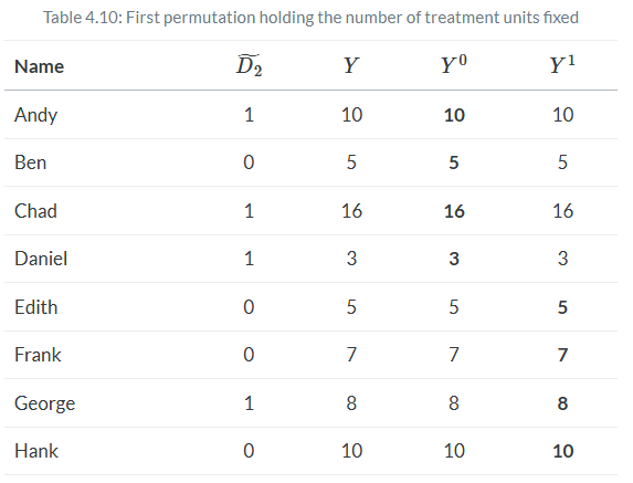
six steps to randomization inference: (1) the choice of the sharp null, (2) the construction of the null, (3) the picking of a different treatment vector, (4) the calculation of the corresponding test statistic for that new treatment vector, (5) the randomization over step 3 as you cycle through a number of new treatment vectors (ideally all possible combinations), and (6) the calculation the exact p-value.

 

We have a particular treatment assignment and a corresponding test statistic. If we assume Fisher’s sharp null, that test statistic is simply a draw from some random process. And if that’s true, then we can shuffle the treatment assignment, calculate a new test statistic and ultimately compare this “fake” test statistic with the real one.

 

The key insight of randomization inference is that under the sharp null, the treatment assignment ultimately does not matter. It explicitly assumes as we go from one assignment to another that the counterfactuals aren’t changing—they are always just equal to the observed outcomes. So the randomization distribution is simply a set of all possible test statistics for each possible treatment assignment vector. The third and fourth steps extend this idea by literally shuffling the treatment assignment and calculating the unique test statistic for each assignment. And as you do this repeatedly (step 5), in the limit you will eventually cycle through all possible combinations that will yield a distribution of test statistics under the sharp null.

 

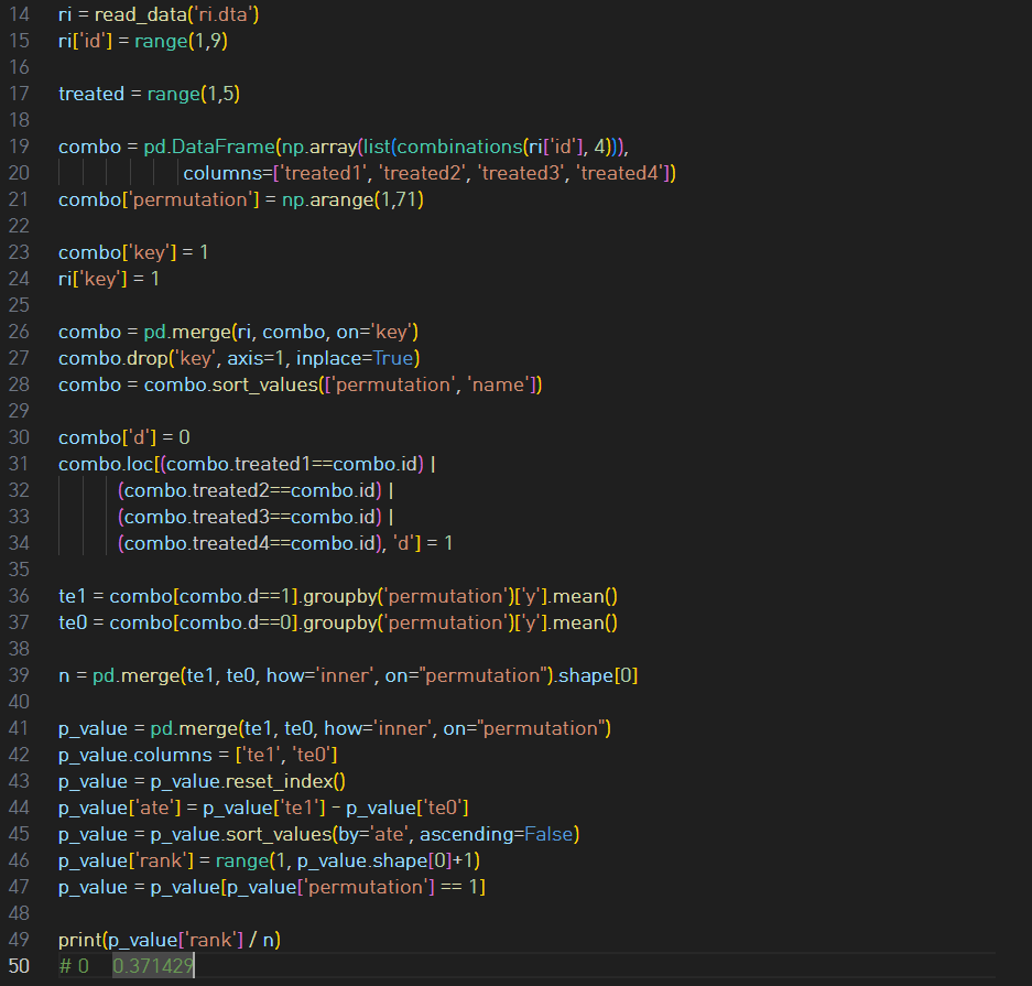
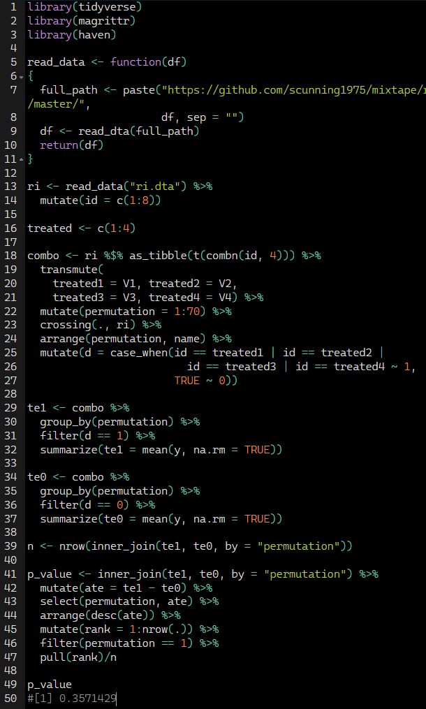
Once you have the entire distribution of test statistics, you can calculate the exact p-value. How? Simple—you rank these test statistics, fit the true effect into that ranking, count the number of fake test statistics that dominate the real one, and divide that number by all possible combinations. Formally, that would be this:

 

Again, we see what is meant by “exact.” These p-values are exact, not approximations. And with a rejection threshold of α—for instance, 0.05—then a randomization inference test will falsely reject the sharp null less than 100×α percent of the time.

---

Calculating p-value

---

Conclusion

We showed that the simple difference in mean outcomes was equal to the sum of the average treatment effect, or the selection bias, and the weighted heterogeneous treatment effect bias. Thus the simple difference-in-mean outcomes estimator is biased unless those second and third terms zero out.

 

One situation in which they zero out is under independence of the treatment, which is when the treatment has been assigned independent of the potential outcomes. When does independence occur? The most commonly confronted situation is under physical randomization of the treatment to the units. Because physical randomization assigns the treatment for reasons that are independent of the potential outcomes, the selection bias zeroes out, as does the heterogeneous treatment effect bias. 

---