code example (1): collider bias

https://mixtape.scunning.com/03-directed_acyclical_graphs

---

Think of a DAG as like a graphical representation of a chain of causal effects. The causal effects are themselves based on some underlying, unobserved structured process, one an economist might call the equilibrium values of a system of behavioral equations, which are themselves nothing more than a model of the world. All of this is captured efficiently using graph notation, such as nodes and arrows. Nodes represent random variables, and those random variables are assumed to be created by some data-generating process. Arrows represent a causal effect between two random variables moving in the intuitive direction of the arrow. The direction of the arrow captures the direction of causality.

 

DAG is meant to describe all causal relationships relevant to the effect of D on Y. What makes the DAG distinctive is both the explicit commitment to a causal effect pathway and the complete commitment to the lack of a causal pathway represented by missing arrows. In other words, a DAG will contain both arrows connecting variables and choices to exclude arrows. And the lack of an arrow necessarily means that you think there is no such relationship in the data—this is one of the strongest beliefs you can hold. A complete DAG will have all direct causal effects among the variables in the graph as well as all common causes of any pair of variables in the graph.

 

At this point, you may be wondering where the DAG comes from. It’s an excellent question. It may be the question. A DAG is supposed to be a theoretical representation of the state-of-the-art knowledge about the phenomena you’re studying. It’s what an expert would say is the thing itself, and that expertise comes from a variety of sources. Examples include economic theory, other scientific models, conversations with experts, your own observations and experiences, literature reviews, as well as your own intuition and hypotheses.

 

I have included this material in the book because I have found DAGs to be useful for understanding the critical role that prior knowledge plays in identifying causal effects. But there are other reasons too. One, I have found that DAGs are very helpful for communicating research designs and estimators if for no other reason than pictures speak a thousand words. This is, in my experience, especially true for instrumental variables, which have a very intuitive DAG representation. Two, through concepts such as the backdoor criterion and collider bias, a well-designed DAG can help you develop a credible research design for identifying the causal effects of some intervention. As a bonus, I also think a DAG provides a bridge between various empirical schools, such as the structural and reduced form groups. And finally, DAGs drive home the point that assumptions are necessary for any and all identification of causal effects, which economists have been hammering at for years.

 

We care about open backdoor paths because they create systematic, noncausal correlations between the causal variable of interest and the outcome you are trying to study. In regression terms, open backdoor paths introduce omitted variable bias, and for all you know, the bias is so bad that it flips the sign entirely. Our goal, then, is to close these backdoor paths. And if we can close all of the otherwise open backdoor paths, then we can isolate the causal effect of D on Y using one of the research designs and identification strategies discussed in this book. So how do we close a backdoor path?

 

There are two ways to close a backdoor path. First, if you have a confounder that has created an open backdoor path, then you can close that path by conditioning on the confounder. Conditioning requires holding the variable fixed using something like subclassification, matching, regression, or another method. It is equivalent to “controlling for” the variable in a regression. The second way to close a backdoor path is the appearance of a collider along that backdoor path. Since colliders always close backdoor paths, and conditioning on a collider always opens a backdoor path, choosing to ignore the colliders is part of your overall strategy to estimate the causal effect itself. By not conditioning on a collider, you will have closed that backdoor path and that takes you closer to your larger ambition to isolate some causal effect.

 

When all backdoor paths have been closed, we say that you have come up with a research design that satisfies the backdoor criterion. And if you have satisfied the backdoor criterion, then you have in effect isolated some causal effect. But let’s formalize this: a set of variables X satisfies the backdoor criterion in a DAG if and only if X blocks every path between confounders that contain an arrow from D to Y. Let’s review our original DAG involving parental education, background and earnings.

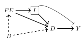
The minimally sufficient conditioning strategy necessary to achieve the backdoor criterion is the control for I, because I appeared as a noncollider along every backdoor path (see earlier). It might literally be no simpler than to run the following regression:

 

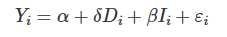
By simply conditioning on I, your estimated δ^ takes on a causal interpretation.

 

The issue of conditioning on a collider is important, so how do we know if we have that problem or not? No data set comes with a flag saying “collider” and “confounder.” Rather, the only way to know whether you have satisfied the backdoor criterion is with a DAG, and a DAG requires a model. It requires in-depth knowledge of the data-generating process for the variables in your DAG, but it also requires ruling out pathways. And the only way to rule out pathways is through logic and models. There is no way to avoid it—all empirical work requires theory to guide it. Otherwise, how do you know if you’ve conditioned on a collider or a noncollider? Put differently, you cannot identify treatment effects without making assumptions.

---

---

 

---

 

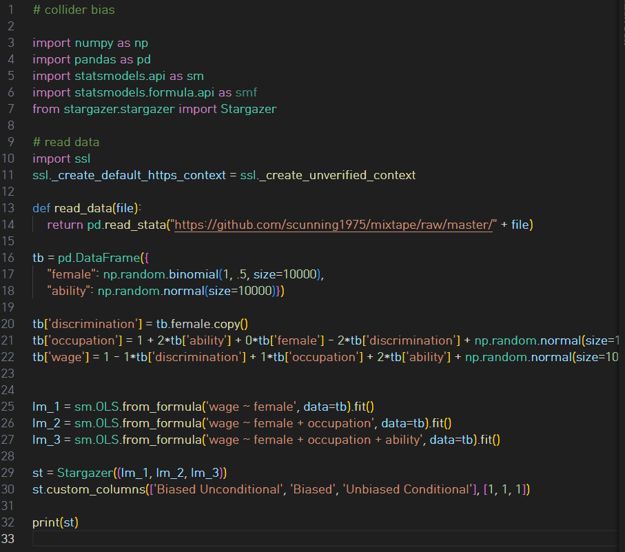
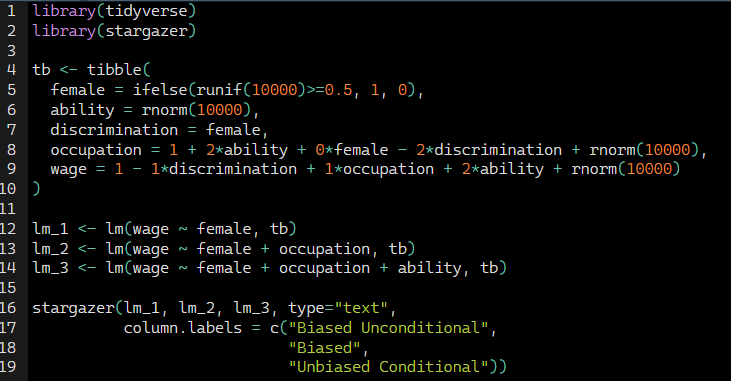
This simulation hard-codes the data-generating process represented by the DAG. Notice that ability is a random draw from the standard normal distribution. Therefore it is independent of female preferences. And then we have our last two generated variables: the heterogeneous occupations and their corresponding wages. Occupations are increasing in unobserved ability but decreasing in discrimination. Wages are decreasing in discrimination but increasing in higher-quality jobs and higher ability. Thus, we know that discrimination exists in this simulation because we are hard-coding it that way with the negative coefficients both the occupation and wage processes.

 

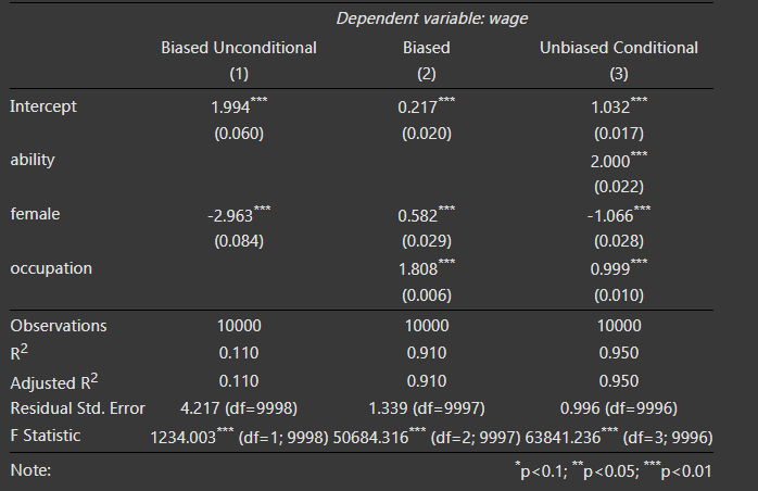
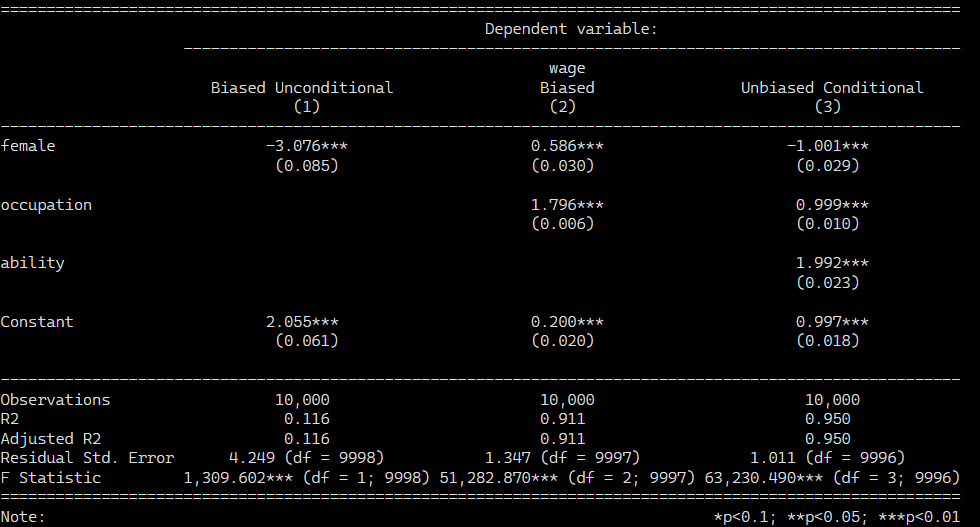
The regression coefficients from the three regressions are presented. First note that when we simply regress wages onto gender, we get a large negative effect, which is the combination of the direct effect of discrimination on earnings and the indirect effect via occupation. But if we run the regression that Google and others recommend wherein we control for occupation, the sign on gender changes. It becomes positive! We know this is wrong because we hard-coded the effect of gender to be −1! The problem is that occupation is a collider. It is caused by ability and discrimination. If we control for occupation, we open up a backdoor path between discrimination and earnings that is spurious and so strong that it perverts the entire relationship. So only when we control for occupation and ability can we isolate the direct causal effect of gender on wages.

---