code example (6): matching - nearest neighbor covariate

ttps://mixtape.scunning.com/05-matching_and_subclassification#exact-matching

---

Subclassification uses the difference between treatment and control group units and achieves covariate balance by using the K probability weights to weight the averages. The subclassification method is using the raw data, but weighting it so as to achieve balance. We are weighting the differences, and then summing over those weighted differences.

 

What if we estimated δ^ATT by imputing the missing potential outcomes by conditioning on the confounding, observed covariate? Specifically, what if we filled in the missing potential outcome for each treatment unit using a control group unit that was “closest” to the treatment group unit for some X confounder? This would give us estimates of all the counterfactuals from which we could simply take the average over the differences. As we will show, this will also achieve covariate balance. This method is called matching.

 

A simple matching estimator is the following:

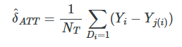
where Yj(i) is the jth unit matched to the ith unit based on the jth being “closest to” the ith unit for some X covariate. 

 

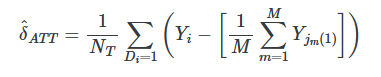
However many matches M that we find, we would assign the average outcome (1/M) as the counterfactual for the treatment group unit.

 

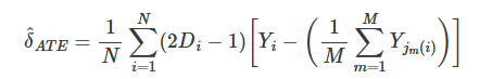
when estimating the ATE, we are filling in both missing control group units like before and missing treatment group units. If observation i is treated, in other words, then we need to fill in the missing Yi0 using the control matches, and if the observation i is a control group unit, then we need to fill in the missing Yi1 using the treatment group matches. The estimator is below.

---

 

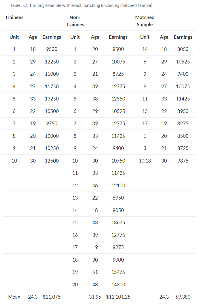
The two groups were different in ways that were likely a direction function of potential outcomes. This means that the independence assumption was violated. Assuming that treatment assignment was conditionally random, then matching on X created an exchangeable set of observations—the matched sample—and what characterized this matched sample was balance.

---

Nearest neighbor covariate matching

But what if you couldn’t find another unit with that exact same value? Then you’re in the world of approximate matching.

 

What does it mean for one unit’s covariate to be “close” to someone else’s? Furthermore, what does it mean when there are multiple covariates with measurements in multiple dimensions?

 

When the number of matching covariates is more than one, we need a new definition of distance to measure closeness. We begin with the simplest measure of distance, the Euclidean distance:

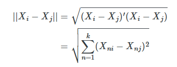
The problem with this measure of distance is that the distance measure itself depends on the scale of the variables themselves. For this reason, researchers typically will use some modification of the Euclidean distance, such as the normalized Euclidean distance, or they’ll use a wholly different alternative distance. The normalized Euclidean distance is a commonly used distance, and what makes it different is that the distance of each variable is scaled by the variable’s variance. The distance is measured as:

Thus, if there are changes in the scale of X, these changes also affect its variance, and so the normalized Euclidean distance does not change.

 

Finally, there is the Mahalanobis distance, which like the normalized Euclidean distance measure, is a scale-invariant distance metric. It is:

 

Basically, more than one covariate creates a lot of headaches. Not only does it create the curse-of-dimensionality problem; it also makes measuring distance harder. All of this creates some challenges for finding a good match in the data.

 

As you can see in each of these distance formulas, there are sometimes going to be matching discrepancies. Sometimes Xi≠Xj.  Sometimes the discrepancies are small, sometimes zero, sometimes large. But, as they move away from zero, they become more problematic for our estimation and introduce bias.

 

How severe is this bias? First, the good news. What we know is that the matching discrepancies tend to converge to zero as the sample size increases—which is one of the main reasons that approximate matching is so data greedy. It demands a large sample size for the matching discrepancies to be trivially small. But what if there are many covariates? The more covariates, the longer it takes for that convergence to zero to occur. Basically, if it’s hard to find good matches with an X that has a large dimension, then you will need a lot of observations as a result. The larger the dimension, the greater likelihood of matching discrepancies, and the more data you need. So you can take that to the bank—most likely, your matching problem requires a large data set in order to minimize the matching discrepancies.

---

Bias correction

Speaking of matching discrepancies, what sorts of options are available to us, putting aside seeking a large data set with lots of controls? Well, enter stage left, Abadie and Imbens (2011), who introduced bias-correction techniques with matching estimators when there are matching discrepancies in finite samples.

 

matching is biased because of these poor matching discrepancies. So let’s derive this bias. First, we write out the sample ATT estimate, and then we subtract out the true ATT. So:

Now consider the implications if the number of covariates is large. First, the difference between Xi and Xj(i) converges to zero slowly. This therefore makes the difference μ0(Xi)−μ(Xj(i)) converge to zero very slowly. Third, E[NT(μ0(Xi)−μ0(Xj(i)))∣D=1] may not converge to zero. And fourth, E[NT(δ^ATT−δATT)] may not converge to zero.

 

As you can see, the bias of the matching estimator can be severe depending on the magnitude of these matching discrepancies. However, one piece of good news is that these discrepancies are observed. We can see the degree to which each unit’s matched sample has severe mismatch on the covariates themselves. Second, we can always make the matching discrepancy small by using a large donor pool of untreated units to select our matches, because recall, the likelihood of finding a good match grows as a function of the sample size, and so if we are content to estimating the ATT, then increasing the size of the donor pool can get us out of this mess.

 

But let’s say we can’t do that and the matching discrepancies are large. Then we can apply bias-correction methods to minimize the size of the bias.

 

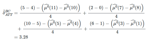
Note that the total bias is made up of the bias associated with each individual unit i. Thus, each treated observation contributes μ0(Xi)−μ0(Xj(i)) to the overall bias. The bias-corrected matching is the following estimator:

where μ^0(X) is an estimate of E[Y∣X=x,D=0] using, for example, OLS.

---

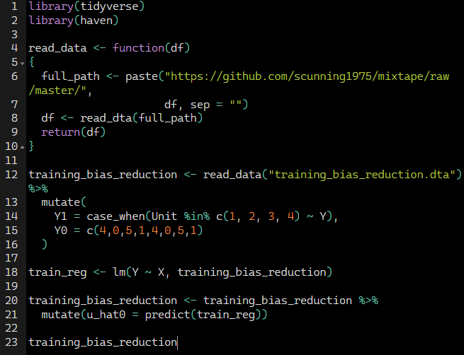
When we regress Y onto X and D, we get the following estimated coefficients:

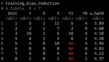
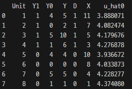
This gives us the outcomes, treatment status, and predicted values.

---