code example (7): matching - propensity score methods

https://mixtape.scunning.com/05-matching_and_subclassification#exact-matching

---

Propensity score methods

propensity score matching is an application used when a conditioning strategy can satisfy the backdoor criterion. But how exactly is it implemented? Propensity score matching takes those necessary covariates, estimates a maximum likelihood model of the conditional probability of treatment (usually a logit or probit so as to ensure that the fitted values are bounded between 0 and 1), and uses the predicted values from that estimation to collapse those covariates into a single scalar called the propensity score. All comparisons between the treatment and control group are then based on that value.

 

The idea with propensity score methods is to compare units who, based on observables, had very similar probabilities of being placed into the treatment group even though those units differed with regard to actual treatment assignment. If conditional on X, two units have the same probability of being treated, then we say they have similar propensity scores, and all remaining variation in treatment assignment is due to chance. And insofar as the two units A and B have the same propensity score of 0.6, but one is the treatment group and one is not, and the conditional independence assumption credibly holds in the data, then differences between their observed outcomes are attributable to the treatment.

 

another assumption needed for this procedure, and that’s the common support assumption. Common support simply requires that there be units in the treatment and control group across the estimated propensity score. We had common support for 0.6 because there was a unit in the treatment group (A) and one in the control group (B) for 0.6. In ways that are connected to this, the propensity score can be used to check for covariate balance between the treatment group and control group such that the two groups become observationally equivalent.

 

I cannot emphasize this enough—this method, like regression more generally, only has value for your project if you can satisfy the backdoor criterion by conditioning on X. If you cannot satisfy the backdoor criterion in your data, then the propensity score does not assist you in identifying a causal effect. At best, it helps you better understand issues related to balance on observables (but not unobservables). It is absolutely critical that your DAG be, in other words, credible, defensible, and accurate, as you depend on those theoretical relationships to design the appropriate identification strategy.

---

Example: NSW job-training program

NSW was a randomized job-training program; therefore, the independence assumption was satisfied. So calculating average treatment effects was straightforward—it’s the simple difference in means estimator.

 

Remember, randomization means that the treatment was independent of the potential outcomes, so simple difference in means identifies the average treatment effect.

 

Lalonde evaluated the econometric estimators’ performance by trading out the experimental control group data with data on the non-experimental control group drawn from the population of US citizens.

 

Table shows the effect of the treatment when comparing the treatment group to the experimental control group. The baseline difference in real earnings between the two groups was negligible. The treatment group made $39 more than the control group in the pre-treatment period without controls and $21 less in the multivariate regression model, but neither is statistically significant. But the post-treatment difference in average earnings was between $798 and $886.

 

Table also shows the results he got when he used the non-experimental data as the comparison group. Here I report his results when using one sample from the PSID and one from the CPS, although in his original paper he used three of each. In nearly every point estimate, the effect is negative. The one exception is the difference-in-differences model which is positive, small, and insignificant.

 

So why is there such a stark difference when we move from the NSW control group to either the PSID or CPS? The reason is because of selection bias:

In other words, it’s highly likely that the real earnings of NSW participants would have been much lower than the non-experimental control group’s earnings. As you recall from our decomposition of the simple difference in means estimator, the second form of bias is selection bias, and if E[Y0∣D=1]<E[Y0∣D=0], this will bias the estimate of the ATE downward (e.g., estimates that show a negative effect).

 

a violation of independence also implies that covariates will be unbalanced across the propensity score—something we call the balancing property.

 

Table 5.12 illustrates this showing the mean values for each covariate for the treatment and control groups, where the control is the 15,992 observations from the CPS. As you can see, the treatment group appears to be very different on average from the control group CPS sample along nearly every covariate listed. 

 

In short, the two groups are not exchangeable on observables (and likely not exchangeable on unobservables either).

 

The first paper to reevaluate Lalonde (1986) using propensity score methods was Dehejia and Wahba (1999). Their interest was twofold. First, they wanted to examine whether propensity score matching could be an improvement in estimating treatment effects using non-experimental data. And second, they wanted to show the diagnostic value of propensity score matching. The authors used the same non-experimental control group data sets from the CPS and PSID as Lalonde (1986) did.

 

Let’s walk through this, and what they learned from each of these steps. First, the authors estimated the propensity score using maximum likelihood modeling. Once they had the estimated propensity score, they compared treatment units to control units within intervals of the propensity score itself. This process of checking whether there are units in both treatment and control for intervals of the propensity score is called checking for common support.

 

One easy way to check for common support is to plot the number of treatment and control group observations separately across the propensity score with a histogram. Dehejia and Wahba (1999) did this using both the PSID and CPS samples and found that the overlap was nearly nonexistent, but here I’ll focus on their CPS sample. The overlap was so bad that they opted to drop 12,611 observations in the control group because their propensity scores were outside the treatment group range. Also, a large number of observations have low propensity scores, evidenced by the fact that the first bin contains 2,969 comparison units. Once this “trimming” was done, the overlap improved, though still wasn’t great.

 

We learn some things from this kind of diagnostic, though. We learn, for one, that the selection bias on observables is probably extreme if for no other reason than the fact that there are so few units in both treatment and control for given values of the propensity score. When there is considerable bunching at either end of the propensity score distribution, it suggests you have units who differ remarkably on observables with respect to the treatment variable itself. Trimming around those extreme values has been a way of addressing this when employing traditional propensity score adjustment techniques.

 

With estimated propensity score in hand, Dehejia and Wahba (1999) estimated the treatment effect on real earnings 1978 using the experimental treatment group compared with the non-experimental control group. The treatment effect here differs from what we found in Lalonde because Dehejia and Wahba (1999) used a slightly different sample. Still, using their sample, they find that the NSW program caused earnings to increase between $1,672 and $1,794 depending on whether exogenous covariates were included in a regression. Both of these estimates are highly significant.

 

The first two columns labeled “unadjusted” and “adjusted” represent OLS regressions with and without controls. Without controls, both PSID and CPS estimates are extremely negative and precise. This, again, is because the selection bias is so severe with respect to the NSW program. When controls are included, effects become positive and imprecise for the PSID sample though almost significant at 5% for CPS. But each effect size is only about half the size of the true effect.

Table 5.13 shows the results using propensity score weighting or matching. As can be seen, the results are a considerable improvement over Lalonde (1986). I won’t review every treatment effect the authors calculated, but I will note that they are all positive and similar in magnitude to what they found in columns 1 and 2 using only the experimental data.

 

Finally, the authors examined the balance between the covariates in the treatment group (NSW) and the various non-experimental (matched) samples in Table 5.14. In the next section, I explain why we expect covariate values to balance along the propensity score for the treatment and control group after trimming the outlier propensity score units from the data. Table 5.14 shows the sample means of characteristics in the matched control sample versus the experimental NSW sample (first row). Trimming on the propensity score, in effect, helped balance the sample. Covariates are much closer in mean value to the NSW sample after trimming on the propensity score.

 

The propensity score is the fitted values of the logit model. Put differently, we used the estimated coefficients from that logit regression to estimate the conditional probability of treatment, assuming that probabilities are based on the cumulative logistic distribution:

As I said earlier, the propensity score used the fitted values from the maximum likelihood regression to calculate each unit’s conditional probability of treatment regardless of actual treatment status. The propensity score is just the predicted conditional probability of treatment or fitted value for each unit. It is advisable to use maximum likelihood when estimating the propensity score so that the fitted values are in the range [0,1]. We could use a linear probability model, but linear probability models routinely create fitted values below 0 and above 1, which are not true probabilities since 0≤p≤1.

 

The definition of the propensity score is the selection probability conditional on the confounding variables; p(X)=Pr(D=1∣X). Recall that we said there are two identifying assumptions for propensity score methods. The first assumption is CIA. That is, (Y0,Y1)⊥⊥D∣X. It is not testable, because the assumption is based on unobservable potential outcomes. The second assumption is called the common support assumption. That is, 0<Pr(D=1∣X)<1. This simply means that for any probability, there must be units in both the treatment group and the control group. The conditional independence assumption simply means that the backdoor criterion is met in the data by conditioning on a vector X. Or, put another way, conditional on X, the assignment of units to the treatment is as good as random.

 

Common support is required to calculate any particular kind of defined average treatment effect, and without it, you will just get some kind of weird weighted average treatment effect for only those regions that do have common support. The reason it is “weird” is that average treatment effect doesn’t correspond to any of the interesting treatment effects the policymaker needed. Common support requires that for each value of X, there is a positive probability of being both treated and untreated, or 0<Pr(Di=1∣Xi)<1. This implies that the probability of receiving treatment for every value of the vector X is strictly within the unit interval. Common support ensures there is sufficient overlap in the characteristics of treated and untreated units to find adequate matches. Unlike CIA, the common support requirement is testable by simply plotting histograms or summarizing the data. Here we do that two ways: by looking at the summary statistics and by looking at a histogram. Let’s start with looking at a distribution in table form before looking at the histogram.

 

The mean value of the propensity score for the treatment group is 0.43, and the mean for the CPS control group is 0.007. The 50th percentile for the treatment group is 0.4, but the control group doesn’t reach that high a number until the 99th percentile. Let’s look at the distribution of the propensity score for the two groups using a histogram now.

These two simple diagnostic tests show what is going to be a problem later when we use inverse probability weighting. The probability of treatment is spread out across the units in the treatment group, but there is a very large mass of nearly zero propensity scores in the CPS. How do we interpret this? What this means is that the characteristics of individuals in the treatment group are rare in the CPS sample. This is not surprising given the strong negative selection into treatment. These individuals are younger, less likely to be married, and more likely to be uneducated and a minority. The lesson is, if the two groups are significantly different on background characteristics, then the propensity scores will have grossly different distributions by treatment status. We will discuss this in greater detail later.

 

For now, let’s look at the treatment parameter under both assumptions.

 

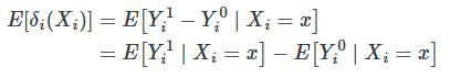
The conditional independence assumption allows us to make the following substitution,

 

and same for the other term. Common support means we can estimate both terms. Therefore, under both assumptions:

 

From these assumptions we get the propensity score theorem, which states that under CIA

 

where p(X)=Pr(D=1∣X), the propensity score. In English, this means that in order to achieve independence, assuming CIA, all we have to do is condition on the propensity score. Conditioning on the propensity score is enough to have independence between the treatment and the potential outcomes.

 

This is an extremely valuable theorem because stratifying on X tends to run into the sparseness-related problems (i.e., empty cells) in finite samples for even a moderate number of covariates. But the propensity scores are just a scalar. So stratifying across a probability is going to reduce that dimensionality problem.

 

Like the omitted variable bias formula for regression, the propensity score theorem says that you need only control for covariates that determine the likelihood a unit receives the treatment. But it also says something more than that. It technically says that the only covariate you need to condition on is the propensity score. All of the information from the X matrix has been collapsed into a single number: the propensity score.

 

A corollary of the propensity score theorem, therefore, states that given CIA, we can estimate average treatment effects by weighting appropriately the simple difference in means.

 

This all works if we match on the propensity score and then calculate differences in means. Direct propensity score matching works in the same way as the covariate matching we discussed earlier (e.g., nearest-neighbor matching), except that we match on the score instead of the covariates directly.

 

Because the propensity score is a function of X, we know

Therefore, conditional on the propensity score, the probability that D=1 does not depend on X any longer. That is, D and X are independent of one another conditional on the propensity score.

 

So from this we also obtain the balancing property of the propensity score:

 

which states that conditional on the propensity score, the distribution of the covariates is the same for treatment as it is for control group units. See this in the following DAG:

Notice that there exist two paths between X and D. There’s the direct path of X→p(X)→D, and there’s the backdoor path X→Y←D. The backdoor path is blocked by a collider, so there is no systematic correlation between X and D through it. But there is systematic correlation between X and D through the first directed path. But, when we condition on p(X), the propensity score, notice that D and X are statistically independent. This implies that D⊥⊥X∣p(X), which implies

This is something we can directly test, but note the implication: conditional on the propensity score, treatment and control should on average be the same with respect to X. In other words, the propensity score theorem implies balanced observable covariates.