01. Introduction To Causality

https://matheusfacure.github.io/python-causality-handbook/landing-page.html

---

Answering a Different Kind of Question

Machine Learning is currently very good at answering the type of question of the prediction kind. As Ajay Agrawal, Joshua Gans, and Avi Goldfarb put it in the book Prediction Machines, “the new wave of artificial intelligence does not actually bring us intelligence but instead a critical component of intelligence - prediction”. We can do all sorts of beautiful things with machine learning. The only requirement is that we frame our problems as prediction ones. Want to translate from English to Portuguese? Then build an ML model that predicts Portuguese sentences when given English sentences. Want to recognize faces? Then create an ML model that predicts the presence of a face in a subsection of a picture. Want to build a self-driving car? Then make one ML model to predict the direction of the wheel and the pressure on the brakes and accelerator when presented with images and sensors from the surroundings of a car.

 

However, ML is not a panacea. It can perform wonders under rigid boundaries and still fail miserably if its data deviates a little from what the model is accustomed to. To give another example from Prediction Machines, “in many industries, low prices are associated with low sales. For example, in the hotel industry, prices are low outside the tourist season, and prices are high when demand is highest and hotels are full. Given that data, a naive prediction might suggest that increasing the price would lead to more rooms sold.”

 

ML is notoriously bad at this inverse causality type of problem. They require us to answer “what if” questions, which economists call counterfactuals. What would happen if I used another price instead of this price I’m currently asking for my merchandise? What would happen if I do a low sugar one instead of this low-fat diet I’m in? If you work in a bank, giving credit, you will have to figure out how changing the customer line changes your revenue. Or, if you work in the local government, you might be asked to figure out how to make the schooling system better. Should you give tablets to every kid because the era of digital knowledge tells you to? Or should you build an old-fashioned library?

 

At the heart of these questions, there is a causal inquiry we wish to know the answer to. Causal questions permeate everyday problems, like figuring out how to make sales go up. Still, they also play an essential role in dilemmas that are very personal and dear to us: do I have to go to an expensive school to be successful in life (does education cause earnings)? Does immigration lower my chances of getting a job (does immigration causes unemployment to go up)? Does money transfer to the poor lower the crime rate? It doesn’t matter the field you are in. It is very likely you had or will have to answer some type of causal question. Unfortunately for ML, we can’t rely on correlation-type predictions to tackle them.

 

Answering this kind of question is more challenging than most people appreciate. Your parents have probably repeated to you that “association is not causation”, “association is not causation”. But actually, explaining why that is the case is a bit more involved. This is what this introduction to causal inference is all about. As for the rest of this book, it will be dedicated to figuring out how to make association be causation.

---

When Association IS Causation

Intuitively, we kind of know why the association is not causation. If someone tells you that schools that give tablets to their students perform better than those that don’t, you can quickly point out that it is probably the case that those schools with the tablets are wealthier. As such, they would do better than average even without the tablets. Because of this, we can’t conclude that giving tablets to kids during classes will cause an increase in their academic performance. We can only say that tablets in school are associated with high academic performance, as measured by ENEM (sort of the SAT in Brazil, which stands for National High School Exam):

The treatment here doesn’t need to be a medicine or anything from the medical field. Instead, it is just a term we will use to denote some intervention for which we want to know the effect. In our case, the treatment is giving tablets to students. As a side note, you might sometimes see D instead of T to denote the treatment.

 

Now, let’s call Yi the observed outcome variable for unit i.

 

The outcome is our variable of interest. We want to know if the treatment has any influence in it. In our tablet example, it would be the academic performance.

 

Here is where things get interesting. The fundamental problem of causal inference is that we can never observe the same unit with and without treatment. 

 

To wrap our heads around this, we will talk a lot in term of potential outcomes. They are potential because they didn’t actually happen. Instead they denote what would have happened in the case some treatment was taken. We sometimes call the potential outcome that happened, factual, and the one that didn’t happen, counterfactual.

 

 

 Y1i is the academic performance for student i if he or she is in a classroom with tablets. Whether this is or not the case, it doesn’t matter for Y1i. It is the same regardless. If student i gets the tablet, we can observe Y1i. If not, we can observe Y0i. Notice how in this last case, Y1i is still defined, we just can’t see it. In this case, it is a counterfactual potential outcome.

 

With potential outcomes, we can define the individual treatment effect:

 

Of course, due to the fundamental problem of causal inference, we can never know the individual treatment effect because we only observe one of the potential outcomes. For the time being, let’s focus on something easier than estimating the individual treatment effect. Instead, lets focus on the average treatment effect, which is defined as follows.

 

Another easier quantity to estimate is the average treatment effect on the treated:

 

Now, I know we can’t see both potential outcomes, but just for the sake of argument, let’s suppose we could. Say we collect data on 4 schools. We know if they gave tablets to its students and their score on some annual academic tests. Here, tablets are the treatment, so T=1 if the school provides tablets to its kids. Y will be the test score.

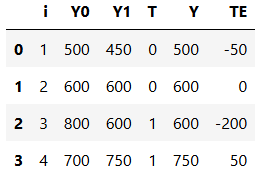
The ATE here would be the mean of the last column, that is, of the treatment effect:

 

This would mean that tablets reduced the academic performance of students, on average, by 50 points. The ATT here would be the mean of the last column when T=1:

 

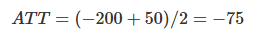
This is saying that, for the schools that were treated, the tablets reduced the academic performance of students, on average, by 75 points. Of course we can never know this. In reality, the table above would look like this:

 

This is surely not ideal, you might say, but can’t I still take the mean of the treated and compare it to the mean of the untreated? In other words, can’t I just do ATE=(600+750)/2−(500+600)/2=125? Well, no! Notice how different the results are. You’ve just committed the gravest sin of mistaking association for causation. To understand why let’s look into the main enemy of causal inference.

---

Bias

Bias is what makes association different from causation. Fortunately, it can be easily understood with our intuition. Let’s recap our tablets in the classroom example. When confronted with the claim that schools that give tablets to their kids achieve higher test scores, we can refute it by saying those schools will probably achieve higher test scores anyway, even without the tablets. That is because they probably have more money than the other schools; hence they can pay better teachers, afford better classrooms, etc. In other words, it is the case that treated schools (with tablets) are not comparable with untreated schools.

 

Using potential outcome notation is to say that Y0 of the treated is different from the Y0 of the untreated. Remember that the Y0 of the treated is counterfactual. We can’t observe it, but we can reason about it. In this particular case, we can even leverage our understanding of how the world works to go even further. We can say that, probably, Y0 of the treated is bigger than Y0 of the untreated schools. That is because schools that can afford to give tablets to their kids can also afford other factors that contribute to better test scores.

 

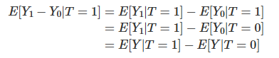
With this in mind, we can show with elementary math why it is the case that association is not causation. Association is measured by E[Y|T=1]−E[Y|T=0]. In our example, this is the average test score for the schools with tablets minus the average test score for those without them. On the other hand, causation is measured by E[Y1−Y0].

 

Let’s take the association measurement and replace the observed outcomes with the potential outcomes to see how they relate. For the treated, the observed outcome is Y1. For the untreated, the observed outcome is Y0.

 

Now, let’s add and subtract E[Y0|T=1]. This is a counterfactual outcome. It tells what would have been the outcome of the treated, had they not received the treatment.

 

Finally, we reorder the terms, merge some expectations, and lo and behold:

 

This simple piece of math encompasses all the problems we will encounter in causal questions. I cannot stress how important it is that you understand every aspect of it. Let’s break it down into some of its implications. First, this equation tells why the association is not causation. As we can see, the association is equal to the treatment effect on the treated plus a bias term. The bias is given by how the treated and control group differ before the treatment, in case neither of them has received the treatment. We can now say precisely why we are suspicious when someone tells us that tablets in the classroom boost academic performance. We think that, in this example, E[Y0|T=0]<E[Y0|T=1], that is, schools that can afford to give tablets to their kids are better than those that can’t, regardless of the tablets treatment.

 

Why does this happen? We will talk more about that once we enter confounding, but for now, you can think of bias arising because many things we can’t control are changing together with the treatment. As a result, the treated and untreated schools don’t differ only on the tablets. They also differ on the tuition cost, location, teachers… For us to say that tablets in the classroom increase academic performance, we would need for schools with and without them to be, on average, similar to each other.

 

Now that we understand the problem let’s look at the solution. We can also say what would be necessary to make association equal to causation. If E[Y0|T=0]=E[Y0|T=1], then, association IS CAUSATION! Understanding this is not just remembering the equation. There is a strong intuitive argument here. To say that E[Y0|T=0]=E[Y0|T=1] is to say that treatment and control group are comparable before the treatment. Or, when the treated had not been treated, if we could observe its Y0, its outcome would be the same as the untreated. Mathematically, the bias term would vanish:

 

Also, if the treated and the untreated only differ on the treatment itself, then, E[Y0|T=0]=E[Y0|T=1] and we have that the causal impact on the treated is the same as in the untreated (because they are very similar).

 

In this case, the difference in means BECOMES the causal effect:

 

Additionally, if the treated and the untreated only differ on the treatment itself, we also have E[Y1|T=0]=E[Y1|T=1], that is, we make sure that both treated and control groups respond similarly to the treatment. Now, besides being exchangeable prior to the treatment, treated and untreated are also exchangeable after the treatment. In this case, E[Y1−Y0|T=1]=E[Y1−Y0|T=0] and

 

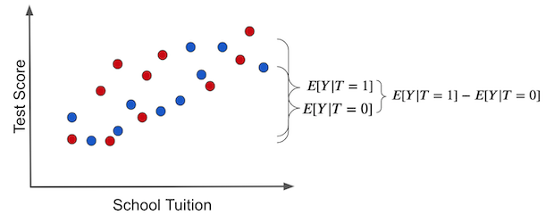
Once again, this is so important that I think it is worth going over it again, now with pretty pictures. If we make a simple average comparison between the treatment and the untreated group, this is what we get (blue dots didn’t receive the treatment, that is, the tablet):

 

Notice how the difference in outcomes between the two groups can have two causes:

1. The treatment effect. The increase in test scores is caused by giving kids tablets.
2. Some of the differences in test scores can be due to tuition prices for better education. In this case, treated and untreated differ because the treated have a much higher tuition price. Other differences between the treatment and untreated are NOT the treatment itself.

The individual treatment effect is the difference between the unit’s outcome and another theoretical outcome that the same unit would have if it got the alternative treatment. The actual treatment effect can only be obtained if we have godlike powers to observe the potential outcome, like the left figure below. These are the counterfactual outcomes and are denoted in a light color.

 

In the right plot, we depicted the bias that we’ve talked about before. We get the bias if we set everyone to not receive the treatment. In this case, we are only left with the T0 potential outcome. Then, we see how the treated and untreated groups differ. If they do, something other than the treatment is causing the treated and untreated to be different. This something is the bias and is what shadows the actual treatment effect.

 

Now, contrast this with a hypothetical situation where there is no bias. Suppose that tablets are randomly assigned to schools. In this situation, rich and poor schools have the same chance of receiving the treatment. Treatment would be well distributed across the tuition spectrum.

 

In this case, the difference in the outcome between treated and untreated IS the average causal effect. This happens because there is no other source of difference between treatment and untreated other than the treatment itself. All the differences we see must be attributed to it. Another way to say this is that there is no bias.

 

If we set everyone to not receive the treatment so that we only observe the Y0s, we would find no difference between the treated and untreated groups.

 

This is the herculean task causal inference is all about. It is about finding clever ways of removing bias and making the treated and the untreated comparable so that all the difference we see is only the average treatment effect. Ultimately, causal inference is about figuring out how the world works, stripped of all delusions and misinterpretations. And now that we understand this, we can move forward to mastering some of the most powerful methods to remove bias, the weapons of the Brave and True, to identify the causal effect.

---

Key Ideas

So far, we’ve seen that association is not causation. Most importantly, we’ve seen precisely why it isn’t and how we can make association be causation. We’ve also introduced the potential outcome notation as a way to wrap our heads around causal reasoning. With it, we saw statistics as two possible realities: one in which the treatment is given and another in which it is not. But unfortunately, we can only measure one of them, where the fundamental problem of causal inference lies.

 

We will see some basic techniques to estimate the causal effect, starting with the golden standard of a randomized trial. I’ll also review some statistical concepts as we go. I’ll end with a quote often used in causal inference classes, taken from a kung-fu series:

---