Scaling Monosemanticity: Extracting Interpretable Features from Claude 3 Sonnet

앞서서 sparse autoencoder로 one-layer transformer에서 monosemantic feature를 추출할 수 있음을 보였다. 

 

이제 sparse autoencoder를 scaling up한다. 

Claude 3 Sonnet에서 monosemantic하고 model의 behavior를 설명할 수 있는 interpretable한 feature를 extracting하는데 성공한다.

 

feature를 manupulate함으로써 model behavior를 steering할 수 있다.

< Takeaway >

1. Sparse autoencoders produce interpretable features for large models.

2. Scaling laws can be used to guide the training of sparse autoencoders.

3. The resulting features are highly abstract: multilingual, multimodal, and generalizing between concrete and abstract references.

4. There appears to be a systematic relationship between the frequency of concepts and the dictionary size needed to resolve features for them.

5. Features can be used to steer large models (see e.g. Influence on Behavior).

---

https://transformer-circuits.pub/2024/scaling-monosemanticity/umap.html?targetId=34m_31164353

Feature UMAP

Decoder space가 얼마나 다양한 feature들을 cover하는지 살펴볼수 있다.

가까이에 놓인 feature들은 유사한 concepts를 가진다. 

 

(embedding space와 유사하다는 생각을 했다).

 

https://transformer-circuits.pub/2024/scaling-monosemanticity/index.html#assessing-sophisticated

Scaling Monosemanticity: Extracting Interpretable Features from Claude 3 Sonnet

---

1. Scaling Dictionary Learning to Claude 3 Sonnet

Our general approach to understanding Claude 3 Sonnet is based on the linear representation hypothesis and the superposition hypothesis.

The linear representation hypothesis suggests that neural networks represent meaningful concepts – referred to as features – as directions in their activation spaces.

 

The superposition hypothesis accepts the idea of linear representations and further hypothesizes that neural networks use the existence of almost-orthogonal directions in high-dimensional spaces to represent more features than there are dimensions.

Based on these hypotheses, use a a specific approximation of dictionary learning called a sparse autoencoder which appears to be very effective for transformer language models.

---

(1) Sparse Autoencoders

Our Goal is to decompose the activations of a model (Claude 3 Sonnet) into more interpretable pieces. We do so by training a sparse autoencoder (SAE) on the model activations.

SAEs are an instance of a family of “sparse dictionary learning” algorithms that seek to decompose data into a weighted sum of sparsely active components.

Our SAE consists of two layers.

 

The first layer (“encoder”) maps the activity to a higher-dimensional layer via a learned linear transformation followed by a ReLU nonlinearity.

 

We refer to the units of this high-dimensional layer as “features.”

 

The second layer (“decoder”) attempts to reconstruct the model activations via a linear transformation of the feature activations.

 

The model is trained to minimize a combination of (1) reconstruction error and (2) an L1 regularization penalty on the feature activations, which incentivizes sparsity.

Once the SAE is trained, it provides us with an approximate decomposition of the model’s activations into a linear combination of “feature directions” (SAE decoder weights) with coefficients equal to the feature activations. 

 

The sparsity penalty ensures that, for many given inputs to the model, a very small fraction of features will have nonzero activations. Thus, for any given token in any given context, the model activations are “explained” by a small set of active features (out of a large pool of possible features). 

* Training

---

(2) SAE experiments

* Applying SAEs to residual stream activations halfway through the model (i.e. at the “middle layer”)

 

* Trained three SAEs of varying sizes: 1,048,576 (~1M), 4,194,304 (~4M), and 33,554,432 (~34M) features.

 

* For all three SAEs, the average number of features active (i.e. with nonzero activations) on a given token was fewer than 300, and the SAE reconstruction explained at least 65% of the variance of the model activations.

 

* At the end of training, defined “dead” features as those which were not active over a sample of 10^7 tokens. The proportion of dead features was roughly 2% for the 1M SAE, 35% for the 4M SAE, and 65% for the 34M SAE. 

---

(3) Scaling Laws

Training SAEs on larger models is computationally intensive. It is important to understand (1) the extent to which additional compute improves dictionary learning results, and (2) how that compute should be allocated to obtain the highest-quality dictionary possible for a given computational budget.

 

Though we lack a gold-standard method of assessing the quality of a dictionary learning run, we have found that the loss function we use during training – a weighted combination of reconstruction mean-squared error (MSE) and an L1 penalty on feature activations – is a useful proxy, conditioned on a reasonable choice of the L1 coefficient. That is, we have found that dictionaries with low loss values (using an L1 coefficient of 5) tend to produce interpretable features and to improve other metrics of interest (the L0 norm, and the number of dead or otherwise degenerate features). 

 

With this proxy, we can treat dictionary learning as a standard machine learning problem, to which we can apply the “scaling laws” framework for hyperparameter optimization.

 

In an SAE, compute usage primarily depends on two key hyperparameters: the number of features being learned, and the number of steps used to train the autoencoder (which maps linearly to the amount of data used, as we train the SAE for only one epoch). The compute cost scales with the product of these parameters if the input dimension and other hyperparameters are held constant.

 

We were also interested in tracking the compute-optimal values of the loss function and parameters of interest; that is, the lowest loss that can be achieved using a given compute budget, and the number of training steps and features that achieve this minimum.

 

Given the compute-optimal choice of training steps and number of features, loss decreases approximately according to a power law with respect to compute.

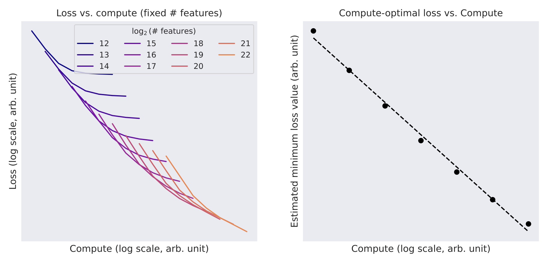
As the compute budget increases, the optimal allocations of FLOPS to training steps and number of features both scale approximately as power laws.

 

These analyses used a fixed learning rate. For different compute budgets, we subsequently swept over learning rates at different optimal parameter settings according to the plots above. The inferred optimal learning rates decreased approximately as a power law as a function of compute budget, and we extrapolated this trend to choose learning rates for the larger runs.

---

2. Assessing Feature Interpretability

Demonstrating what the features represent and how they function in the network.

(1) Four Examples of Interpretable Features

 

While these examples suggest interpretations for each feature, more work needs to be done to establish that our interpretations truly capture the behavior and function of the corresponding features.

 

For each feature, we attempt to establish the following claims:

1. When the feature is active, the relevant concept is reliably present in the context (Specificity).
2. Intervening on the feature’s activation produces relevant downstream behavior (influence on behavior).

< Specificity >

It is difficult to rigorously measure the extent to which a concept is present in a text input. To demonstrate specificity, we leverage automated interpretability methods.

 

we additionally find that current-generation models can now more accurately rate text samples according to how well they match a proposed feature interpretation.

 

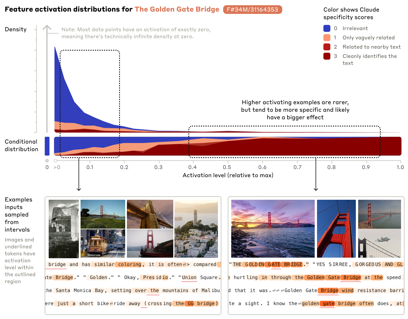
We constructed the following rubric for scoring how a feature’s description relates to the text on which it fires. We then asked Claude 3 Opus to rate feature activations at many tokens on that rubric.

• 0 – The feature is completely irrelevant throughout the context (relative to the base distribution of the internet).
• 1 – The feature is related to the context, but not near the highlighted text or only vaguely related.
• 2 – The feature is only loosely related to the highlighted text or related to the context near the highlighted text.
• 3 – The feature cleanly identifies the activating text.

By scoring examples of activating text, we provide a measure of specificity for each feature.

 

Below we show distributions of feature activations (excluding zero activations) for the four features mentioned above, along with example text and image inputs that induce low and high activations.

 

* a Golden Gate Bridge feature 34M/31164353. Its greatest activations are essentially all references to the bridge, and weaker activations also include related tourist attractions, similar bridges, and other monuments.

 

* a brain sciences feature 34M/9493533 activates on discussions of neuroscience books and courses, as well as cognitive science, psychology, and related philosophy.

 

* a feature that strongly activates for various kinds of transit infrastructure 1M/3 including trains, ferries, tunnels, bridges, and even wormholes.

 

* feature 1M/887839  responds to popular tourist attractions including the Eiffel Tower, the Tower of Pisa, the Golden Gate Bridge, and the Sistine Chapel.

 

To quantify specificity, we used Claude 3 Opus to automatically score examples that activate these features according to the rubric above, with roughly 1000 activations of the feature drawn from the dataset used to train the dictionary learning model.

 

We plot the frequency of each rubric score as a function of the feature’s activation level. We see that inputs that induce strong feature activations are all judged to be highly consistent with the proposed interpretation.

 

< Influence on Behavior >

whether our interpretations of features accurately describe their influence on model behavior, we experiment with feature steering, where we “clamp” specific features of interest to artificially high or low values during the forward pass.

 

Feature steering is remarkably effective at modifying model outputs in specific, interpretable ways. It can be used to modify the model’s demeanor, preferences, stated goals, and biases; to induce it to make specific errors; and to circumvent model safeguards. We find this compelling evidence that our interpretations of features line up with how they are used by the model.

 

For instance, we see that clamping the Golden Gate Bridge feature 34M/31164353 to 10× its maximum activation value induces thematically-related model behavior. In this example, the model starts to self-identify as the Golden Gate Bridge! Similarly, clamping the Transit infrastructure feature 1M/3 to 5× its maximum activation value causes the model to mention a bridge when it otherwise would not. In each case, the downstream influence of the feature appears consistent with our interpretation of the feature.

 

---

(2) Sophisticated Features

< Code Error Feature >

 

As a first experiment, we input a prompt with bug-free code and clamped the feature to a large positive activation. We see that the model proceeds to hallucinate an error message:

 

We can also intervene to clamp this feature to a large negative activation. Doing this for code that does contain a bug causes the model to predict what the code would have produced if the bug was not there!

< Features Representing Functions >

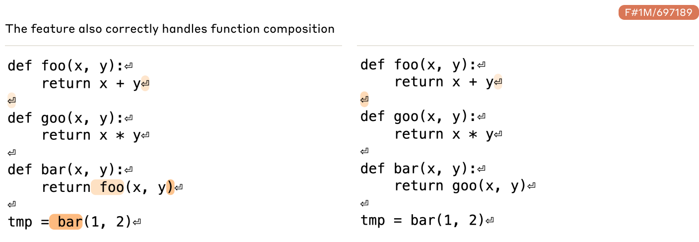
We also discovered features that track specific function definitions and references to them in code. A particularly interesting example is an addition feature 1M/697189, which activates on names of functions that add numbers. For example, this feature fires on “bar” when it is defined to perform addition, but not when it is defined to perform multiplication. Moreover, it fires at the end of any function definition that implements addition.

 

Remarkably, this feature even correctly handles function composition, activating in response to functions that call other functions that perform addition. In the following example, on the left, we redefine “bar” to call “foo”, therefore inheriting its addition operation and causing the feature to fire. On the right, “bar” instead calls the multiply operation from “goo”, and the feature does not fire.

 

We also verified that this feature is in fact involved in the model’s computation of addition-related functions. For instance, this feature is among the top ten features with strongest attributions  when the model is asked to execute a block of code involving an addition function.

 

Thus this feature appears to represent the function of addition being performed by the model. To further test this hypothesis, we experimented with clamping the feature to be active on code that does not involve addition. When we do so, we find that the model is “tricked” into believing that it has been asked to execute an addition.

---

3. Feature Survey

The features we find in Sonnet are rich and diverse. One challenge is that we have millions of features.

 

Scaling feature exploration is an important open problem.

 

we have made some progress in characterizing the space of features, aided by automated interpretability.

 

1. local structure of features, which are often organized in geometrically-related clusters that share a semantic relationship.

 

2. global properties of features, such as how comprehensively they cover a given topic or category.

 

3. examine some categories of features we uncovered through manual inspection.

---

(1) Exploring Feature Neighborhoods

Here we walk through the local neighborhoods of several features of interest across the 1M, 4M and 34M SAEs, with closeness measured by the cosine similarity of the feature vectors. We find that this consistently surfaces features that share a related meaning or context.

< Golden Gate Bridge Feature >

Focusing on a small neighborhood around the Golden Gate Bridge feature 34M/31164353. Overall, it appears that distance in decoder space maps roughly onto relatedness in concept space, often in interesting and unexpected ways.

 

We also find evidence of feature splitting, a phenomenon in which features in smaller SAEs “split” into multiple features in a larger SAE, which are geometrically close and semantically related to the original feature, but represent more specific concepts. For instance, a “San Francisco” feature in the 1M SAE splits into two features in the 4M SAE and eleven fine-grained features in the 34M SAE.

 

In addition to feature splitting, we also see examples in which larger SAEs contain features that represent concepts not captured by features in smaller SAEs. For instance, there is a group of earthquake features from the 4M and 34M SAEs that has no analog in this neighborhood in the 1M SAE, nor do any of the nearest 1M SAE features seem related.

< Immunology Feature >

Immunology feature 1M/533737. We see several distinct clusters within this neighborhood.

These results are consistent with the trend identified above, in which nearby features in dictionary vector space touch on similar concepts.

< Inner Conflict Feature >

Inner Conflict feature 1M/284095.

While this neighborhood does not cleanly separate out into clusters, we still find that different subregions are associated with different themes.

---

(2) Feature Completeness

* The breadth and completeness with which our features cover the space of concepts.

For instance, does the model have a feature corresponding to every major world city? To study questions like this, we used Claude to search for features which fired on members of particular families of concepts/terms. Specifically:

1. We pass a prompt with the relevant concept (e.g. “The physicist Richard Feynman”) to the model and see which features activate on the final token.
2. We then take the top five features by activation magnitude and run them through our automated interpretability pipeline, asking Sonnet to provide explanations of what those features fire on.
3. We then look at each of the top 5 explanations and a human rater judges whether the concept, or some subset of the concept, is specifically indicated by the model-generated explanation as the most important part of the feature.

We find increasing coverage of concepts as we increase the number of features, though even in the 34M SAE we see evidence that the set of features we uncovered is an incomplete description of the model’s internal representations. For instance, we confirmed that Claude 3 Sonnet can list all of the London boroughs when asked, and in fact can name tens of individual streets in many of the areas. However, we could only find features corresponding to about 60% of the boroughs in the 34M SAE. This suggests that the model contains many more features than we have found, which may be able to be extracted with even larger SAEs.

* What determines whether a feature corresponding to a concept is present in our SAEs.

Representation in our dictionaries is closely tied with the frequency of the concept in the training data.

 

For instance, chemical elements which are mentioned often in the training data almost always have corresponding features in our dictionary, while those which are mentioned rarely or not at all do not.

 

A consistent tendency for the larger SAEs to have features for concepts that are rarer in the training data, with the rough “threshold” frequency required for a feature to be present being similar across categories.

 

This finding gives us some handle on the SAE scale at which we should expect a concept-specific feature to appear – if a concept is present in the training data only once in a billion tokens, then we should expect to need a dictionary with on the order of a billion alive features in order to find a feature which uniquely represents that specific concept. Importantly, not having a feature dedicated to a particular concept does not mean that the reconstructed activations do not contain information about that concept, as the model can use multiple related features compositionally to reference a specific concept.

 

This also informs how much data we should expect to need in order to train larger dictionaries – if we assume that the SAE needs to see data corresponding to a feature a certain fixed number of times during training in order to learn it, then the amount of SAE training data needed to learn N features would be proportional to N.

---

(3) Feature Categories

< Person Features >

We find many features corresponding to famous individuals, which are active on descriptions of those people as well as relevant historical context.

< Country Features >

Many of these features fire not just on the country name itself, but also when the country is being described.

< Basic Code Features >

a number of features that represent different syntax elements or other low-level concepts in code, which give the impression of syntax highlighting when visualized together 

< List Position Features >

---

4. Features as Computational Intermediates

Features let us examine the intermediate computation that the model uses to produce an output. We observe that in prompts where intermediate computation is required, we find active features corresponding to some of the expected intermediate results.

 

A simple strategy for efficiently identifying causally important features for a model's output is to compute attributions, which are local linear approximations of the effect of turning a feature off at a specific location on the model's next-token prediction.

 

We also perform feature ablations, where we clamp a feature’s value to zero at a specific token position during a forward pass, which measures the full, potentially nonlinear causal effect of that feature’s activation in that position on the model output. 

 

We find that the middle layer residual stream of the model contains a range of features causally implicated in the model's completion.

---

(1) Emotional Inferences

As an example, we consider the following incomplete prompt:

 

John says, "I want to be alone right now." John feels (completion: sad − happy)

 

To continue this text, the model must parse the quote from John, identify his state of mind, and then translate that into a likely feeling.

 

If we sort features by either their attribution or their ablation effect on the completion “sad” (with respect to a baseline completion of “happy”), the top two features are:

• 1M/22623 – This feature fires when someone expresses a need or desire to be alone or have personal time and space, as in “she would probably want some time to herself”. This is active from the word “alone” onwards. This suggests the model has gotten the gist of John's expression.
• 1M/781220 – This feature detects expressions of sadness, crying, grief, and related emotional distress or sorrow, as in “the inconsolable girl sobs”. This is active on “John feels”. This suggests the model has inferred what someone who says they are alone might be feeling.

If we look at dataset examples, we can see that they align with these interpretations.

 

The fact that both features contribute to the final output indicates that the model has partially predicted a sentiment from John's statement (the second feature) but will do more downstream processing on the content of his statement (as represented by the first feature) as well.

---