Placebos in DD

https://mixtape.scunning.com/09-difference_in_differences#inference

---

1. The Importance of Placesbos in DD

There are several tests of the validity of a DD strategy. I have already discussed one—comparability between treatment and control groups on observable pre-treatment dynamics. Next, I will discuss other credible ways to evaluate whether estimated causal effects are credible by emphasizing the use of placebo falsification.

 

The idea of placebo falsification is simple. Say that you are finding some negative effect of the minimum wage on low-wage employment. Is the hypothesis true if we find evidence in favor? Maybe, maybe not. Maybe what would really help, though, is if you had in mind an alternative hypothesis and then tried to test that alternative hypothesis. If you cannot reject the null on the alternative hypothesis, then it provides some credibility to your original analysis. For instance, maybe you are picking up something spurious, like cyclical factors or other unobservables not easily captured by a time or state fixed effects. So what can you do?

 

One candidate placebo falsification might simply be to use data for an alternative type of worker whose wages would not be affected by the binding minimum wage. For instance, minimum wages affect employment and earnings of low-wage workers as these are the workers who literally are hired based on the market wage. Without some serious general equilibrium gymnastics, the minimum wage should not affect the employment of higher wage workers, because the minimum wage is not binding on high wage workers. Since high- and low-wage workers are employed in very different sectors, they are unlikely to be substitutes. This reasoning might lead us to consider the possibility that higher wage workers might function as a placebo.

 

There are two ways you can go about incorporating this idea into our analysis. Many people like to be straightforward and simply fit the same DD design using high wage employment as the outcome. If the coefficient on minimum wages is zero when using high wage worker employment as the outcome, but the coefficient on minimum wages for low wage workers is negative, then we have provided stronger evidence that complements the earlier analysis we did when on the low wage workers. But there is another method that uses the within-state placebo for identification called the difference-in-differences-in-differences (“triple differences”). 

---

2. Triple differences

In our earlier analysis, we assumed that the only thing that happened to New Jersey after it passed the minimum wage was a common shock, T, but what if there were state-specific time shocks such as NJ_t or PA_t? Then even DD cannot recover the treatment effect. Let’s see for ourselves using a modification of the simple minimum-wage table from earlier, which will include the within-state workers who hypothetically were untreated by the minimum wage—the “high-wage workers.”

 

Before the minimum-wage increase, low- and high-wage employment in New Jersey is determined by a group-specific New Jersey fixed effect (e.g., NJ_h). The same is true for Pennsylvania. But after the minimum-wage hike, four things change in New Jersey: national trends cause employment to change by T; New Jersey-specific time shocks change employment by NJ_t; generic trends in low-wage workers change employment by l_t; and the minimum-wage has some unknown effect D. We have the same setup in Pennsylvania except there is no minimum wage, and Pennsylvania experiences its own time shocks.

 

Now if we take first differences for each set of states, we only eliminate the state fixed effect. The first difference estimate for New Jersey includes the minimum-wage effect, D, but is also hopelessly contaminated by confounders (i.e., T+NJ_t+l_t). So we take a second difference for each state, and doing so, we eliminate two of the confounders: T disappears and NJ_t disappears. But while this DD strategy has eliminated several confounders, it has also introduced new ones (i.e., (l_t−h_t)). This is the final source of selection bias that triple differences are designed to resolve. But, by differencing Pennsylvania’s second difference from New Jersey, the (l_t−h_t) is deleted and the minimum-wage effect is isolated.

 

Now, this solution is not without its own set of unique parallel-trends assumptions. But one of the parallel trends here I’d like you to see is the l_t−h_t term. This parallel trends assumption states that the effect can be isolated if the gap between high- and low-wage employment would’ve evolved similarly in the treatment state counterfactual as it did in the historical control states. And we should probably provide some credible evidence that this is true with leads and lags in an event study as before.

---

3. State-mandated maternity benefits

The triple differences design was first introduced by Gruber (1994) in a study of state-level policies providing maternity benefits. I present his main results in Table 9.3. Notice that he uses as his treatment group married women of childbearing age in treatment and control states, but he also uses a set of placebo units (older women and single men 20–40) as within-state controls. He then goes through the differences in means to get the difference-in-differences for each set of groups, after which he calculates the DDD as the difference between these two difference-in-differences.

 

Ideally when you do a DDD estimate, the causal effect estimate will come from changes in the treatment units, not changes in the control units. That’s precisely what we see in Gruber (1994): the action comes from changes in the married women age 20–40 (−0.062); there’s little movement among the placebo units (−0.008). Thus when we calculate the DDD, we know that most of that calculation is coming from the first DD, and not so much from the second. We emphasize this because DDD is really just another falsification exercise, and just as we would expect no effect had we done the DD on this placebo group, we hope that our DDD estimate is also based on negligible effects among the control group.

 

What we have done up to now is show how to use sample analogs and simple differences in means to estimate the treatment effect using DDD. But we can also use regression to control for additional covariates that perhaps are necessary to close backdoor paths and so forth. What does that regression equation look like? Both the regression itself, and the data structure upon which the regression is based, are complicated because of the stacking of different groups and the sheer number of interactions involved. Estimating a DDD model requires estimating the following regression:

 

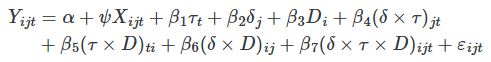
where the parameter of interest is β7. First, notice the additional subscript, j. This j indexes whether it’s the main category of interest (e.g., low-wage employment) or the within-state comparison group (e.g., high-wage employment). This requires a stacking of the data into a panel structure by group, as well as state. Second, the DDD model requires that you include all possible interactions across the group dummy δj, the post-treatment dummy τt and the treatment state dummy Di. The regression must include each dummy independently, each individual interaction, and the triple differences interaction. One of these will be dropped due to multicollinearity, but I include them in the equation so that you can visualize all the factors used in the product of these terms.

---