(1/2) Causal Representation Learning

https://arxiv.org/pdf/2102.11107

---

Abstract

The two fields of machine learning and graphical causality arose and developed separately. However, there is now cross-pollination and increasing interest in both fields to benefit from the advances of the other. In the present paper, we review fundamental concepts of causal inference and relate them to crucial open problems of machine learning, including transfer and generalization, thereby assaying how causality can contribute to modern machine learning research. This also applies in the opposite direction: we note that most work in causality starts from the premise that the causal variables are given. A central problem for AI and causality is, thus, causal representation learning, the discovery of high-level causal variables from low-level observations. Finally, we delineate some implications of causality for machine learning and propose key research areas at the intersection of both communities.

---

1. Introduction

If we compare what machine learning can do to what animals accomplish, we observe that the former is rather limited at some crucial feats where natural intelligence excels. These include transfer to new problems and any form of generalization that is not from one data point to the next (sampled from the same distribution), but rather from one problem to the next — both have been termed generalization, but the latter is a much harder form thereof, sometimes referred to as horizontal, strong, or out-of-distribution generalization. This shortcoming is not too surprising, given that machine learning often disregards information that animals use heavily: interventions in the world, domain shifts, temporal structure — by and large, we consider these factors a nuisance and try to engineer them away. In accordance with this, the majority of current successes of machine learning boil down to large scale pattern recognition on suitably collected independent and identically distributed (i.i.d.) data.

 

To illustrate the implications of this choice and its relation to causal models, we start by highlighting key research challenges.

a) Issue 1 – Robustness:

With the widespread adoption of deep learning approaches in computer vision [101, 140], natural language processing [54], and speech recognition [85], a substantial body of literature explored the robustness of the prediction of state-of-the-art deep neural network architectures. The underlying motivation originates from the fact that in the real world there is often little control over the distribution from which the data comes from. In computer vision [75, 228], changes in the test distribution may, for instance, come from aberrations like camera blur, noise or compression quality [106, 129, 170, 206], or from shifts, rotations, or viewpoints [7, 11, 63, 282]. Motivated by this, new benchmarks were proposed to specifically test generalization of classification and detection methods with respect to simple algorithmically generated interventions like spatial shifts, blur, changes in brightness or contrast [106, 170], time consistency [94, 227], control over background and rotation [11], as well as images collected in multiple environments [19]. Studying the failure modes of deep neural networks from simple interventions has the potential to lead to insights into the inductive biases of state-of-the-art architectures. So far, there has been no definitive consensus on how to solve these problems, although progress has been made using data augmentation, pre-training, self-supervision, and architectures with suitable inductive biases w.r.t. a perturbation of interest [233, 59, 63, 137, 170, 206]. It has been argued [188] that such fixes may not be sufficient, and generalizing well outside the i.i.d. setting requires learning not mere statistical associations between variables, but an underlying causal model. The latter contains the mechanisms giving rise to the observed statistical dependences, and allows to model distribution shifts through the notion of interventions [183, 237, 218, 34, 188, 181].

b) Issue 2 – Learning Reusable Mechanisms:

Infants’ understanding of physics relies upon objects that can be tracked over time and behave consistently [52, 236]. Such a representation allows children to quickly learn new tasks as their knowledge and intuitive understanding of physics can be re-used [15, 52, 144, 250]. Similarly, intelligent agents that robustly solve real-world tasks need to re-use and re-purpose their knowledge and skills in novel scenarios. Machine learning models that incorporate or learn structural knowledge of an environment have been shown to be more efficient and generalize better [14, 10, 16, 84, 197, 212, 8, 274, 26, 76, 83, 141, 157, 177, 211, 245, 258, 272, 57, 182]. In a modular representation of the world where the modules correspond to physical causal mechanisms, many modules can be expected to behave similarly across different tasks and environments. An agent facing a new environment or task may thus only need to adapt a few modules in its internal representation of the world [220, 84]. When learning a causal model, one should thus require fewer examples to adapt as most knowledge, i.e., modules, can be re-used without further training.

c) A Causality Perspective:

Causation is a subtle concept that cannot be fully described using the language of Boolean logic [151] or that of probabilistic inference; it requires the additional notion of intervention [237, 183]. The manipulative definition of causation [237, 183, 118] focuses on the fact that conditional probabilities (“seeing people with open umbrellas suggests that it is raining”) cannot reliably predict the outcome of an active intervention (“closing umbrellas does not stop the rain”). Causal relations can also be viewed as the components of reasoning chains [151] that provide predictions for situations that are very far from the observed distribution and may even remain purely hypothetical [163, 183] or require conscious deliberation [128]. In that sense, discovering causal relations means acquiring robust knowledge that holds beyond the support of an observed data distribution and a set of training tasks, and it extends to situations involving forms of reasoning.

 

Our Contributions: In the present paper, we argue that causality, with its focus on representing structural knowledge about the data generating process that allows interventions and changes, can contribute towards understanding and resolving some limitations of current machine learning methods. This would take the field a step closer to a form of artificial intelligence that involves thinking in the sense of Konrad Lorenz, i.e., acting in an imagined space [163]. Despite its success, statistical learning provides a rather superficial description of reality that only holds when the experimental conditions are fixed. Instead, the field of causal learning seeks to model the effect of interventions and distribution changes with a combination of data-driven learning and assumptions not already included in the statistical description of a system. The present work reviews and synthesizes key contributions that have been made to this end:

 

• We describe different levels of modeling in physical systems in Section II and present the differences between causal and statistical models in Section III. We do so not only in terms of modeling abilities but also discuss the assumptions and challenges involved.

 

• We expand on the Independent Causal Mechanisms (ICM) principle as a key component that enables the estimation of causal relations from data in Section IV. In particular, we state the Sparse Mechanism Shift hypothesis as a consequence of the ICM principle and discuss its implications for learning causal models.

 

• We review existing approaches to learn causal relations from appropriate descriptors (or features) in Section V. We cover both classical approaches and modern re-interpretations based on deep neural networks, with a focus on the underlying principles that enable causal discovery.

 

• We discuss how useful models of reality may be learned from data in the form of causal representations, and discuss several current problems of machine learning from a causal point of view in Section VI.

 

• We assay the implications of causality for practical machine learning in Section VII. Using causal language, we revisit robustness and generalization, as well as existing common practices such as semi-supervised learning, self-supervised learning, data augmentation, and pre-training. We discuss examples at the intersection between causality and machine learning in scientific applications and speculate on the advantages of combining the strengths of both fields to build a more versatile AI.

---

2. Levels of Causal Modeling

The gold standard for modeling natural phenomena is a set of coupled differential equations modeling physical mechanisms responsible for the time evolution. This allows us to predict the future behavior of a physical system, reason about the effect of interventions, and predict statistical dependencies between variables that are generated by coupled time evolution. It also offers physical insights, explaining the functioning of the system, and lets us read off its causal structure. To this end, consider the coupled set of differential equations

with initial value x(t0) = x0. The Picard–Lindelöf theorem states that at least locally, if f is Lipschitz, there exists a unique solution x(t). This implies in particular that the immediate future of x is implied by its past values.

 

If we formally write this in terms of infinitesimal differentials dt and dx = x(t + dt) − x(t), we get:

 

From this, we can ascertain which entries of the vector x(t) mathematically determine the future of others x(t + dt). This tells us that if we have a physical system whose physical mechanisms are correctly described using such an ordinary differential equation (1), solved for dx / dt (i.e., the derivative only appears on the left-hand side), then its causal structure can be directly read off.1

 

(1Note that this requires that the differential equation system describes the causal physical mechanisms. If, in contrast, we considered a set of differential equations that phenomenologically correctly describe the time evolution of a system without capturing the underlying mechanisms (e.g., due to unobserved confounding, or a form of course-graining that does not preserve the causal structure [207]), then (2) may not be causally meaningful [221, 190].)

 

While a differential equation is a rather comprehensive description of a system, a statistical model can be viewed as a much more superficial one. It often does not refer to dynamic processes; instead, it tells us how some of the variables allow prediction of others as long as experimental conditions do not change. E.g., if we drive a differential equation system with certain types of noise, or we average over time, then it may be the case that statistical dependencies between components of x emerge, and those can then be exploited by machine learning. Such a model does not allow us to predict the effect of interventions; however, its strength is that it can often be learned from observational data, while a differential equation usually requires an intelligent human to come up with it. Causal modeling lies in between these two extremes. Like models in physics, it aims to provide understanding and predict the effect of interventions. However, causal discovery and learning try to arrive at such models in a data-driven way, replacing expert knowledge with weak and generic assumptions. The overall situation is summarized in Table I, adapted from [188]. Below, we address some of the tasks listed in Table I in more detail.

A. Predicting in the i.i.d. setting

Statistical models are a superficial description of reality as they are only required to model associations. For a given set of input examples X and target labels Y , we may be interested in approximating P(Y |X) to answer questions like: “what is the probability that this particular image contains a dog?” or “what is the probability of heart failure given certain diagnostic measurements (e.g., blood pressure) carried out on a patient?”. Subject to suitable assumptions, these questions can be provably answered by observing a sufficiently large amount of i.i.d. data from P(X, Y ) [257]. Despite the impressive advances of machine learning, causality offers an under-explored complement: accurate predictions may not be sufficient to inform decision making. For example, the frequency of storks is a reasonable predictor for human birth rates in Europe [168]. However, as there is no direct causal link between those two variables, a change to the stork population would not affect the birth rates, even though a statistical model may predict so. The predictions of a statistical model are only accurate within identical experimental conditions. Performing an intervention changes the data distribution, which may lead to (arbitrarily) inaccurate predictions [183, 237, 218, 188].

B. Predicting Under Distribution Shifts

Interventional questions are more challenging than predictions as they involve actions that take us out of the usual i.i.d. setting of statistical learning. Interventions may affect both the value of a subset of causal variables and their relations. For example, “is increasing the number of storks in a country going to boost its human birth rate?” and “would fewer people smoke if cigarettes were more socially stigmatized?”. As interventions change the joint distribution of the variables of interest, classical statistical learning guarantees [257] no longer apply. On the other hand, learning about interventions may allow to train predictive models that are robust against the changes in distribution that naturally happen in the real world. Here, interventions do not need to be deliberate actions to achieve a goal. Statistical relations may change dynamically over time (e.g., people’s preferences and tastes) or there may simply be a mismatch between a carefully controlled training distribution and the test distribution of a model deployed in production. The robustness of deep neural networks has recently been scrutinized and become an active research topic related to causal inference. We argue that predicting under distribution shift should not be reduced to just the accuracy on a test set. If we wish to incorporate learning algorithms into human decision making, we need to trust that the predictions of the algorithm will remain valid if the experimental conditions are changed.

C. Answering Counterfactual Questions

Counterfactual problems involve reasoning about why things happened, imagining the consequences of different actions in hindsight, and determining which actions would have achieved a desired outcome. Answering counterfactual questions can be more difficult than answering interventional questions. However, this may be a key challenge for AI, as an intelligent agent may benefit from imagining the consequences of its actions as well as understanding in retrospect what led to certain outcomes, at least to some degree of approximation.2 We have above mentioned the example of statistical predictions of heart failure. An interventional question would be “how does the probability of heart failure change if we convince a patient to exercise regularly?” A counterfactual one would be “would a given patient have suffered heart failure if they had started exercising a year earlier?”. As we shall discuss below, counterfactuals, or approximations thereof, are especially critical in reinforcement learning. They can enable agents to reflect on their decisions and formulate hypotheses that can be empirically verified in a process akin to the scientific method.

 

2Note that the two types of questions occupy a continuum: to this end, consider a probability which is both conditional and interventional P(A|B, do(C)). If B is the empty set, we have a classical intervention; if B contained all (unobserved) noise terms, we have a counterfactual. If B is not identical to the noise terms, but nevertheless informative about them, we get something in between. For instance, reinforcement learning practitioners may call Q functions as providing counterfactuals, even though they model P(return from t| agent state at time t, do (action at time t)), and therefore closer to an intervention (which is why they can be estimated from data)

D. Nature of Data: Observational, Interventional, (Un)structured

The data format plays a substantial role in which type of relation can be inferred. We can distinguish two axes of data modalities: observational versus interventional, and hand-engineered versus raw (unstructured) perceptual input.

Observational and Interventional Data:

an extreme form of data which is often assumed but seldom strictly available is observational i.i.d. data, where each data point is independently sampled from the same distribution. Another extreme is interventional data with known interventions, where we observe data sets sampled from multiple distributions each of which is the result of a known intervention. In between, we have data with (domain) shifts or unknown interventions. This is observational in the sense that the data is only observed passively, but it is interventional in the sense that there are interventions/shifts, but unknown to us.

Hand Engineered Data vs. Raw Data:

especially in classical AI, data is often assumed to be structured into high-level and semantically meaningful variables which may partially (modulo some variables being unobserved) correspond to the causal variables of the underlying graph. Raw Data, in contrast, is unstructured and does not expose any direct information about causality.

 

While statistical models are weaker than causal models, they can be efficiently learned from observational data alone on both hand-engineered features and raw perceptual input such as images, videos, speech etc. On the other hand, although methods for learning causal structure from observations exist [237, 188, 229, 113, 174, 187, 139, 17, 246, 277, 175, 123, 186, 176, 36, 82, 161], learning causal relations frequently requires collecting data from multiple environments, or the ability to perform interventions [251]. In some cases, it is assumed that all common causes of measured variables are also observed (causal sufficiency).3 Overall, a significant amount of prior knowledge is encoded in which variables are measured. Moving forward, one would hope to develop methods that replace expert data collection with suitable inductive biases and learning paradigms such as meta-learning and self-supervision. If we wish to learn a causal model that is useful for a particular set of tasks and environments, the appropriate granularity of the high-level variables depends on the tasks of interest and on the type of data we have at our disposal, for example which interventions can be performed and what is known about the domain.

 

3There are also algorithms that do not require causal sufficiency [237].

---

3. Causal Models and Inference

As discussed, reality can be modeled at different levels, from the physical one to statistical associations between epiphenomena. In this section, we expand on the difference between statistical and causal modeling and review a formal language to talk about interventions and distribution changes.

A. Methods driven by i.i.d. data

The machine learning community has produced impressive successes with machine learning applications to big data problems [148, 171, 223, 231, 53]. In these successes, there are several trends at work [215]: (1) we have massive amounts of data, often from simulations or large scale human labeling, (2) we use high capacity machine learning systems (i.e., complex function classes with many adjustable parameters), (3) we employ high-performance computing systems, and finally (often ignored, but crucial when it comes to causality) (4) the problems are i.i.d. The latter can be guaranteed by the construction of a task including training and test set (e.g., image recognition using benchmark datasets). Alternatively, problems can be made approximately i.i.d., e.g.. by carefully collecting the right training set for a given application problem, or by methods such as “experience replay” [171] where a reinforcement learning agent stores observations in order to later permute them for the purpose of re-training.

 

For i.i.d. data, strong universal consistency results from statistical learning theory apply, guaranteeing convergence of a learning algorithm to the lowest achievable risk. Such algorithms do exist, for instance, nearest neighbor classifiers, support vector machines, and neural networks [257, 217, 239, 66]. Seen in this light, it is not surprising that we can indeed match or surpass human performance if given enough data. However, current machine learning methods often perform poorly when faced with problems that violate the i.i.d. assumption, yet seem trivial to humans. Vision systems can be grossly misled if an object that is normally recognized with high accuracy is placed in a context that in the training set may be negatively correlated with the presence of the object. Distribution shifts may also arise from simple corruptions that are common in real-world data collection pipelines [9, 106, 129, 170, 206]. An example of this is the impact of socio-economic factors in clinics in Thailand on the accuracy of a detection system for Diabetic Retinopathy [18]. More dramatically, the phenomenon of “adversarial vulnerability” [249] highlights how even tiny but targeted violations of the i.i.d. assumption, generated by adding suitably chosen perturbations to images, imperceptible to humans, can lead to dangerous errors such as confusion of traffic signs. Overall, it is fair to say that much of the current practice (of solving i.i.d. benchmark problems) and most theoretical results (about generalization in i.i.d. settings) fail to tackle the hard open challenge of generalization across problems.

 

To further understand how the i.i.d. assumption is problematic, let us consider a shopping example. Suppose Alice is looking for a laptop rucksack on the internet (i.e., a rucksack with a padded compartment for a laptop). The web shop’s recommendation system suggests that she should buy a laptop to go along with the rucksack. This seems odd because she probably already has a laptop, otherwise she would not be looking for the rucksack in the first place. In a way, the laptop is the cause, and the rucksack is an effect. Now suppose we are told whether a customer has bought a laptop. This reduces our uncertainty about whether she also bought a laptop rucksack, and vice versa —- and it does so by the same amount (the mutual information), so the directionality of cause and effect is lost. However, the directionality is present in the physical mechanisms generating statistical dependence, for instance the mechanism that makes a customer want to buy a rucksack once she owns a laptop.4 Recommending an item to buy constitutes an intervention in a system, taking us outside the i.i.d. setting. We no longer work with the observational distribution, but a distribution where certain variables or mechanisms have changed.

 

4Note that the physical mechanisms take place in time, and if available, time order may provide additional information about causality.

---

B. The Reichenbach Principle: From Statistics to Causality

Reichenbach [198] clearly articulated the connection between causality and statistical dependence. He postulated:

 

Common Cause Principle: if two observables X and Y are statistically dependent, then there exists a variable Z that causally influences both and explains all the dependence in the sense of making them independent when conditioned on Z.

 

As a special case, this variable can coincide with X or Y . Suppose that X is the frequency of storks and Y the human birth rate. If storks bring the babies, then the correct causal graph is X → Y . If babies attract storks, it is X ← Y . If there is some other variable that causes both (such as economic development), we have X ← Z → Y .

 

Without additional assumptions, we cannot distinguish these three cases using observational data. The class of observational distributions over X and Y that can be realized by these models is the same in all three cases. A causal model thus contains genuinely more information than a statistical one.

 

While causal structure discovery is hard if we have only two observables [187], the case of more observables is surprisingly easier, the reason being that in that case, there are nontrivial conditional independence properties [238, 51, 74] implied by causal structure. These generalize the Reichenbach Principle and can be described by using the language of causal graphs or structural causal models, merging probabilistic graphical models and the notion of interventions [237, 183]. They are best described using directed functional parent-child relationships rather than conditionals. While conceptually simple in hindsight, this constituted a major step in the understanding of causality.

---

C. Structural causal models (SCMs)

The SCM viewpoint considers a set of observables (or variables) X1, . . . , Xn associated with the vertices of a directed acyclic graph (DAG). We assume that each observable is the result of an assignment

using a deterministic function fi depending on Xi’s parents in the graph (denoted by PAi) and on an unexplained random variable Ui . Mathematically, the observables are thus random variables, too. Directed edges in the graph represent direct causation, since the parents are connected to Xi by directed edges and through (3) directly affect the assignment of Xi . The noise Ui ensures that the overall object (3) can represent a general conditional distribution P(Xi |PAi), and the set of noises U1, . . . , Un are assumed to be jointly independent. If they were not, then by the Common Cause Principle there should be another variable that causes their dependence, and thus our model would not be causally sufficient.

 

If we specify the distributions of U1, . . . , Un, recursive application of (3) allows us to compute the entailed observational joint distribution P(X1, . . . , Xn). This distribution has structural properties inherited from the graph [147, 183]: it satisfies the causal Markov condition stating that conditioned on its parents, each Xj is independent of its non-descendants.

 

Intuitively, we can think of the independent noises as “information probes” that spread through the graph (much like independent elements of gossip can spread through a social network). Their information gets entangled, manifesting itself in a footprint of conditional dependencies making it possible to infer aspects of the graph structure from observational data using independence testing. Like in the gossip analogy, the footprint may not be sufficiently characteristic to pin down a unique causal structure. In particular, it certainly is not if there are only two observables, since any nontrivial conditional independence statement requires at least three variables. The two-variable problem can be addressed by making additional assumptions, as not only the graph topology leaves a footprint in the observational distribution, but the functions fi do, too. This point is interesting for machine learning, where much attention is devoted to properties of function classes (e.g., priors or capacity measures), and we shall return to it below.

a) Causal Graphical Models:

The graph structure along with the joint independence of the noises implies a canonical factorization of the joint distribution entailed by (3) into causal conditionals that we refer to as the causal (or disentangled) factorization,

While many other entangled factorizations are possible, e.g.,

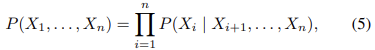
the factorization (4) yields practical computational advantages during inference, which is in general hard, even when it comes to non-trivial approximations [210]. But more interestingly, it is the only one that decomposes the joint distribution into conditionals corresponding to the structural assignments (3). We think of these as the causal mechanisms that are responsible for all statistical dependencies among the observables. Accordingly, in contrast to (5), the disentangled factorization represents the joint distribution as a product of causal mechanisms.

b) Latent variables and Confounders:

Variables in a causal graph may be unobserved, which can make causal inference particularly challenging. Unobserved variables may confound two observed variables so that they either appear statistically related while not being causally related (i.e., neither of the variables is an ancestor of the other), or their statistical relation is altered by the presence of the confounder (e.g., one variable is a causal ancestor for the other, but the confounder is a causal ancestor of both). Confounders may or may not be known or observed.

c) Interventions:

The SCM language makes it straightforward to formalize interventions as operations that modify a subset of assignments (3), e.g., changing Ui , setting fi (and thus Xi) to a constant, or changing the functional form of fi (and thus the dependency of Xi on its parents) [237, 183].

 

Several types of interventions may be possible [62] which can be categorized as: No intervention: only observational data is obtained from the causal model. Hard/perfect: the function in the structural assignment (3) of a variable (or, analogously, of multiple variables) is set to a constant (implying that the value of the variable is fixed), and then the entailed distribution for the modified SCM is computed. Soft/imperfect: the structural assignment (3) for a variable is modified by changing the function or the noise term (this corresponds to changing the conditional distribution given its parents). Uncertain: the learner is not sure which mechanism/variable is affected by the intervention.

 

One could argue that stating the structural assignments as in (3) is not yet sufficient to formulate a causal model. In addition, one should specify the set of possible interventions on the structural causal model. This may be done implicitly via the functional form of structural equations by allowing any intervention over the domain of the mechanisms. This becomes relevant when learning a causal model from data, as the SCM depends on the interventions. Pragmatically, we should aim at learning causal models that are useful for specific sets of tasks of interest [207, 267] on appropriate descriptors (in terms of which causal statements they support) that must either be provided or learned. We will return to the assumptions that allow learning causal models and features in Section IV.

---

D. Difference Between Statistical Models, Causal Graphical Models, and SCMs

 

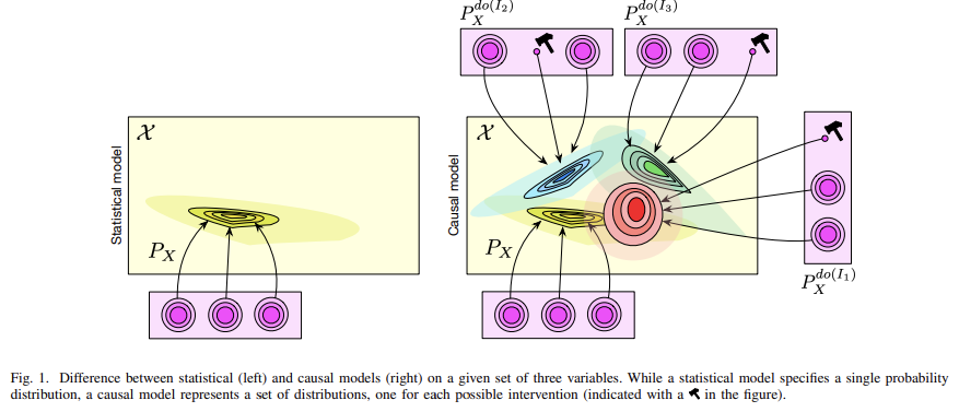
An example of the difference between a statistical and a causal model is depicted in Figure 1. A statistical model may be defined for instance through a graphical model, i.e., a probability distribution along with a graph such that the former is Markovian with respect to the latter (in which case it can be factorized as (4)). However, the edges in a (generic) graphical model do not need to be causal [97]. For instance, the two graphs X1 → X2 → X3 and X1 ← X2 ← X3 imply the same conditional independence(s) (X1 and X3 are independent given X2). They are thus in the same Markov equivalence class, i.e., if a distribution is Markovian w.r.t. one of the graphs, then it also is w.r.t. the other graph. Note that the above serves as an example that the Markov condition is not sufficient for causal discovery. Further assumptions are needed, cf. below and [237, 183, 188].

 

A graphical model becomes causal if the edges of its graph are causal (in which case the graph is referred to as a “causal graph”), cf. (3). This allows to compute interventional distributions as depicted in Figure 1. When a variable is intervened upon, we disconnect it from its parents, fix its value, and perform ancestral sampling on its children.

 

A structural causal model is composed of (i) a set of causal variables and (ii) a set of structural equations with a distribution over the noise variables Ui (or a set of causal conditionals). While both causal graphical models and SCMs allow to compute interventional distributions, only the SCMs allow to compute counterfactuals. To compute counterfactuals, we need to fix the value of the noise variables. Moreover, there are many ways to represent a conditional as a structural assignment (by picking different combinations of functions and noise variables).

a) Causal Learning and Reasoning:

The conceptual basis of statistical learning is a joint distribution P(X1, . . . , Xn) (where often one of the Xi is a response variable denoted as Y ), and we make assumptions about function classes used to approximate, say, a regression E[Y |X]. Causal learning considers a richer class of assumptions, and seeks to exploit the fact that the joint distribution possesses a causal factorization (4). It involves the causal conditionals P(Xi | PAi) (e.g., represented by the functions fi and the distribution of Ui in (3)), how these conditionals relate to each other, and interventions or changes that they admit. Once a causal model is available, either by external human knowledge or a learning process, causal reasoning allows to draw conclusions on the effect of interventions, counterfactuals and potential outcomes. In contrast, statistical models only allow to reason about the outcome of i.i.d. experiments.

---

4. Independent Causal Mechanisms

We now return to the disentangled factorization (4) of the joint distribution P(X1, . . . , Xn). This factorization according to the causal graph is always possible when the Ui are independent, but we will now consider an additional notion of independence relating the factors in (4) to one another.

 

Whenever we perceive an object, our brain assumes that the object and the mechanism by which the information contained in its light reaches our brain are independent. We can violate this by looking at the object from an accidental viewpoint, which can give rise to optical illusions [188]. The above independence assumption is useful because in practice, it holds most of the time, and our brain thus relies on objects being independent of our vantage point and the illumination. Likewise, there should not be accidental coincidences, such as 3D structures lining up in 2D, or shadow boundaries coinciding with texture boundaries. In vision research, this is called the generic viewpoint assumption.

 

If we move around the object, our vantage point changes, but we assume that the other variables of the overall generative process (e.g., lighting, object position and structure) are unaffected by that. This is an invariance implied by the above independence, allowing us to infer 3D information even without stereo vision (“structure from motion”).

 

For another example, consider a dataset that consists of altitude A and average annual temperature T of weather stations [188]. A and T are correlated, which we believe is due to the fact that the altitude has a causal effect on temperature. Suppose we had two such datasets, one for Austria and one for Switzerland. The two joint distributions P(A, T) may be rather different since the marginal distributions P(A) over altitudes will differ. The conditionals P(T|A), however, may be (close to) invariant, since they characterize the physical mechanisms that generate temperature from altitude. This similarity is lost upon us if we only look at the overall joint distribution, without information about the causal structure A → T. The causal factorization P(A)P(T|A) will contain a component P(T|A) that generalizes across countries, while the entangled factorization P(T)P(A|T) will exhibit no such robustness. Cum grano salis, the same applies when we consider interventions in a system. For a model to correctly predict the effect of interventions, it needs to be robust to generalizing from an observational distribution to certain interventional distributions.

 

One can express the above insights as follows [218, 188]:

 

Independent Causal Mechanisms (ICM) Principle. The causal generative process of a system’s variables is composed of autonomous modules that do not inform or influence each other. In the probabilistic case, this means that the conditional distribution of each variable given its causes (i.e., its mechanism) does not inform or influence the other mechanisms.

 

This principle entails several notions important to causality, including separate intervenability of causal variables, modularity and autonomy of subsystems, and invariance [183, 188]. If we have only two variables, it reduces to an independence between the cause distribution and the mechanism producing the effect distribution.

 

Applied to the causal factorization (4), the principle tells us that the factors should be independent in the sense that

 

(a) changing (or performing an intervention upon) one mechanism P(Xi |PAi) does not change any of the other mechanisms P(Xj |PAj ) (i /= j) [218], and

 

(b) knowing some other mechanisms P(Xi |PAi) (i /= j) does not give us information about a mechanism P(Xj |PAj ) [120].

 

This notion of independence thus subsumes two aspects: the former pertaining to influence, and the latter to information.

 

The notion of invariant, autonomous, and independent mechanisms has appeared in various guises throughout the history of causality research [99, 71, 111, 183, 120, 240, 188]. Early work on this was done by Haavelmo [99], stating the assumption that changing one of the structural assignments leaves the other ones invariant. Hoover [111] attributes to Herb Simon the invariance criterion: the true causal order is the one that is invariant under the right sort of intervention. Aldrich [4] discusses the historical development of these ideas in economics. He argues that the “most basic question one can ask about a relation should be: How autonomous is it?” [71, preface]. Pearl [183] discusses autonomy in detail, arguing that a causal mechanism remains invariant when other mechanisms are subjected to external influences. He points out that causal discovery methods may best work “in longitudinal studies conducted under slightly varying conditions, where accidental independencies are destroyed and only structural independencies are preserved.” Overviews are provided by Aldrich [4], Hoover [111], Pearl [183], and Peters et al. [188, Sec. 2.2]. These seemingly different notions can be unified [120, 240].

 

We view any real-world distribution as a product of causal mechanisms. A change in such a distribution (e.g., when moving from one setting/domain to a related one) will always be due to changes in at least one of those mechanisms. Consistent with the implication (a) of the ICM Principle, we state the following hypothesis:

 

Sparse Mechanism Shift (SMS). Small distribution changes tend to manifest themselves in a sparse or local way in the causal/disentangled factorization (4), i.e., they should usually not affect all factors simultaneously.

 

In contrast, if we consider a non-causal factorization, e.g., (5), then many, if not all, terms will be affected simultaneously as we change one of the physical mechanisms responsible for a system’s statistical dependencies. Such a factorization may thus be called entangled, a term that has gained popularity in machine learning [23, 109, 158, 247].

 

The SMS hypothesis was stated in [181, 24, 221, 115], and in earlier form in [218, 279, 220]. An intellectual ancestor is Simon’s invariance criterion, i.e., that the causal structure remains invariant across changing background conditions [235]. The hypothesis is also related to ideas of looking for features that vary slowly [69, 270]. It has recently been used for learning causal models [131], modular architectures [84, 28] and disentangled representations [159].

 

We have informally talked about the dependence of two mechanisms P(Xi |PAi) and P(Xj |PAj ) when discussing the ICM Principle and the disentangled factorization (4). Note that the dependence of two such mechanisms does not coincide with the statistical dependence of the random variables Xi and Xj . Indeed, in a causal graph, many of the random variables will be dependent even if all mechanisms are independent. Also, the independence of the noise terms Ui does not translate into the independence of the Xi . Intuitively speaking, the independent noise terms Ui provide and parameterize the uncertainty contained in the fact that a mechanism P(Xi |PAi) is non-deterministic,5 and thus ensure that each mechanism adds an independent element of uncertainty. In this sense, the ICM Principle contains the independence of the unexplained noise terms in an SCM (3) as a special case.

 

In the ICM Principle, we have stated that independence of two mechanisms (formalized as conditional distributions) should mean that the two conditional distributions do not inform or influence each other. The latter can be thought of as requiring that independent interventions are possible. To better understand the former, we next discuss a formalization in terms of algorithmic independence. In a nutshell, we encode each mechanism as a bit string, and require that joint compression of these strings does not save space relative to independent compressions

 

To this end, first recall that we have so far discussed links between causal and statistical structures. Of the two, the more fundamental one is the causal structure, since it captures the physical mechanisms that generate statistical dependencies in the first place. The statistical structure is an epiphenomenon that follows if we make the unexplained variables random. It is awkward to talk about statistical information contained in a mechanism since deterministic functions in the generic case neither generate nor destroy information. This serves as a motivation to devise an alternative model of causal structures in terms of Kolmogorov complexity [120]. The Kolmogorov complexity (or algorithmic information) of a bit string is essentially the length of its shortest compression on a Turing machine, and thus a measure of its information content. Independence of mechanisms can be defined as vanishing mutual algorithmic information; i.e., two conditionals are considered independent if knowing (the shortest compression of) one does not help us achieve a shorter compression of the other.

 

Algorithmic information theory provides a natural framework for non-statistical graphical models [120, 126]. Just like the latter are obtained from structural causal models by making the unexplained variables Ui random, we obtain algorithmic graphical models by making the Ui bit strings, jointly independent across nodes, and viewing Xi as the output of a fixed Turing machine running the program Ui on the input PAi . Similar to the statistical case, one can define a local causal Markov condition, a global one in terms of d-separation, and an additive decomposition of the joint Kolmogorov complexity in analogy to (4), and prove that they are implied by the structural causal model [120]. Interestingly, in this case, independence of noises and independence of mechanisms coincide, since the independent programs play the role of the unexplained noise terms. This approach shows that causality is not intrinsically bound to statistics.

 

5 In the sense that the mapping from PAi to Xi is described by a non-trivial conditional distribution, rather than by a function.

---