(2/2) Causal Representation Learning

https://arxiv.org/pdf/2102.11107

---

5. Causal Discovery and Machine Learning

Let us turn to the problem of causal discovery from data. Subject to suitable assumptions such as faithfulness [237], one can sometimes recover aspects of the underlying graph6 from observational data by performing conditional independence tests.

 

6One can recover the causal structure up to a Markov equivalence class, where DAGs have the same undirected skeleton and “immoralities” (Xi → Xj ← Xk).

 

However, there are several problems with this approach. One is that our datasets are always finite in practice, and conditional independence testing is a notoriously difficult problem, especially if conditioning sets are continuous and multi-dimensional. So while, in principle, the conditional independencies implied by the causal Markov condition hold irrespective of the complexity of the functions appearing in an SCM, for finite datasets, conditional independence testing is hard without additional assumptions [225]. Recent progress in (conditional) independence testing heavily relies on kernel function classes to represent probability distributions in reproducing kernel Hilbert spaces [90, 91, 73, 278, 60, 191, 42]. The other problem is that in the case of only two variables, the ternary concept of conditional independence collapses and the Markov condition thus has no nontrivial implications.

 

It turns out that both problems can be addressed by making assumptions on function classes. This is typical for machine learning, where it is well-known that finite-sample generalization without assumptions on function classes is impossible. Specifically, although there are universally consistent learning algorithms, i.e., approaching minimal expected error in the infinite sample limit, there are always cases where this convergence is arbitrarily slow. So for a given sample size, it will depend on the problem being learned whether we achieve low expected error, and statistical learning theory provides probabilistic guarantees in terms of measures of complexity of function classes [55, 257].

 

Returning to causality, we provide an intuition why assumptions on the functions in an SCM should be necessary to learn about them from data. Consider a toy SCM with only two observables X → Y . In this case, (3) turns into

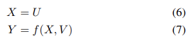
with U ⊥⊥ V . Now think of V acting as a random selector variable choosing from among a set of functions F = {fv(x) ≡ f(x, v) | v ∈ supp(V )}. If f(x, v) depends on v in a non-smooth way, it should be hard to glean information about the SCM from a finite dataset, given that V is not observed and its value randomly selects among arbitrarily different fv.

 

This motivates restricting the complexity with which f depends on V . A natural restriction is to assume an additive noise model

 

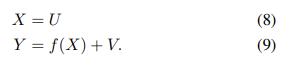
If f in (7) depends smoothly on V , and if V is relatively well concentrated, this can be motivated by a local Taylor expansion argument. It drastically reduces the effective size of the function class — without such assumptions, the latter could depend exponentially on the cardinality of the support of V . Restrictions of function classes not only make it easier to learn functions from data, but it turns out that they can break the symmetry between cause and effect in the two-variable case: one can show that given a distribution over X, Y generated by an additive noise model, one cannot fit an additive noise model in the opposite direction (i.e., with the roles of X and Y interchanged) [113, 174, 187, 139, 17], cf. also [246]. This is subject to certain genericity assumptions, and notable exceptions include the case where U, V are Gaussian and f is linear. It generalizes results of Shimizu et al. [229] for linear functions, and it can be generalized to include non-linear rescalings [277], loops [175], confounders [123], and multi-variable settings [186]. Empirically, there is a number of methods that can detect causal direction better than chance [176], some of them building on the above Kolmogorov complexity model [36], some on generative models [82], and some directly learning to classify bivariate distributions into causal vs. anticausal [161].

 

While restrictions of function classes are one possibility to allow to identify the causal structure, other assumptions or scenarios are possible. So far, we have discussed that causal models are expected to generalize under certain distribution shifts since they explicitly model interventions. By the SMS hypothesis, much of the causal structure is assumed to remain invariant. Hence distribution shifts such as observing a system in different “environments / contexts” can significantly help to identify causal structure [251, 188]. These contexts can come from interventions [218, 189, 192], non-stationary time series [117, 100, 193] or multiple views [89, 115]. The contexts can likewise be interpreted as different tasks, which provide a connection to meta-learning [22, 67, 213].

 

The work of Bengio et al. [24] ties the generalization in meta-learning to invariance properties of causal models, using the idea that a causal model should adapt faster to interventions than purely predictive models. This was extended to multiple variables and unknown interventions in [131], proposing a framework for causal discovery using neural networks by turning the discrete graph search into a continuous optimization problem. While [24, 131] focus on learning a causal model using neural networks with an unsupervised loss, the work of Dasgupta et al. [50] explores learning a causal model using a reinforcement learning agent. These approaches have in common that semantically meaningful abstract representations are given and do not need to be learned from high-dimensional and low-level (e.g., pixel) data.

---

6. Learning Causal Variables

Traditional causal discovery and reasoning assume that the units are random variables connected by a causal graph. However, real-world observations are usually not structured into those units to begin with, e.g., objects in images [162]. Hence, the emerging field of causal representation learning strives to learn these variables from data, much like machine learning went beyond symbolic AI in not requiring that the symbols that algorithms manipulate be given a priori (cf. Bonet and Geffner [33]). To this end, we could try to connect causal variables S1, . . . , Sn to observations

where G is a non-linear function.

 

An example can be seen in Figure 2, where high-dimensional observations are the result of a view on the state of a causal system that is then processed by a neural network to extract high-level variables that are useful on a variety of tasks. Although causal models in economics, medicine, or psychology often use variables that are abstractions of underlying quantities, it is challenging to state general conditions under which coarse-grained variables admit causal models with well-defined interventions [41, 207]. Defining objects or variables that can be causally related amounts to coarse-graining of more detailed models of the world, including microscopic structural equation models [207], ordinary differential equations [173, 208], and temporally aggregated time series [78]. The task of identifying suitable units that admit causal models is challenging for both human and machine intelligence. Still, it aligns with the general goal of modern machine learning to learn meaningful representations of data, where meaningful can include robust, explainable, or fair [142, 133, 276, 130, 260].

 

To combine structural causal modeling (3) and representation learning, we should strive to embed an SCM into larger machine learning models whose inputs and outputs may be high-dimensional and unstructured, but whose inner workings are at least partly governed by an SCM (that can be parameterized with a neural network). The result may be a modular architecture, where the different modules can be individually fine-tuned and re-purposed for new tasks [181, 84] and the SMS hypothesis can be used to enforce the appropriate structure. We visualize an example in Figure 3 where changes are sparse for the appropriate causal variables (the position of the finger and the cube changed as a result of moving the finger), but dense in other representations, for example in the pixel space (as finger and cube move, many pixels change their value). At the extreme, all pixels may change as a result of a sparse intervention, for example, if the camera view or the lighting changes.

 

We now discuss three problems of modern machine learning in the light of causal representation learning.

a) Problem 1 - Learning Disentangled Representations:

We have earlier discussed the ICM Principle implying both the independence of the SCM noise terms in (3) and thus the feasibility of the disentangled representation

as well as the property that the conditionals P(Si | PAi) be independently manipulable and largely invariant across related problems. Suppose we seek to reconstruct such a disentangled representation using independent mechanisms (11) from data, but the causal variables Si are not provided to us a priori. Rather, we are given (possibly high-dimensional) X = (X1, . . . , Xd) (below, we think of X as an image with pixels X1, . . . , Xd) as in (10), from which we should construct causal variables S1, . . . , Sn (n << d) as well as mechanisms, cf. (3),

modeling the causal relationships among the Si . To this end, as a first step, we can use an encoder q : R^d → R^n taking X to a latent “bottleneck” representation comprising the unexplained noise variables U = (U1, . . . , Un). The next step is the mapping f(U) determined by the structural assignments f1, . . . , fn. Finally, we apply a decoder p : R^n → R^d . For suitable n, the system can be trained using reconstruction error to satisfy p ◦ f ◦ q ≈ id on the observed images. If the causal graph is known, the topology of a neural network implementing f can be fixed accordingly; if not, the neural network decoder learns the composition p˜ = p ◦ f. In practice, one may not know f, and thus only learn an autoencoder p˜ ◦ q, where the causal graph effectively becomes an unspecified part of the decoder p˜, possibly aided by a suitable choice of architecture [149].

 

Much of the existing work on disentanglement [109, 158, 159, 256, 157, 135, 202, 61] focuses on independent factors of variation. This can be viewed as the special case where the causal graph is trivial, i.e., ∀i : PAi = ∅ in (12). In this case, the factors are functions of the independent exogenous noise variables, and thus independent themselves.7 However, the ICM Principle is more general and contains statistical independence as a special case.

 

(7For an example to see why this is often not desirable, note that the presence of fork and knife may be statistically dependent, yet we might want a disentangled representation to represent them as separate entities.)

 

Note that the problem of object-centric representation learning [10, 39, 83, 86, 87, 138, 155, 160, 262, 255] can also be considered a special case of disentangled factorization as discussed here. Objects are constituents of scenes that in principle permit separate interventions. A disentangled representation of a scene containing objects should probably use objects as some of the building blocks of an overall causal factorization8 , complemented by mechanisms such as orientation, viewing direction, and lighting.

 

(8Objects can be represented at different levels of granularity [207], i.e. as a single entity or as a composition of other causal variables encoding parts, properties, and other factors of variation.)

 

The problem of recovering the exogenous noise variables is ill-defined in the i.i.d. case as there are infinitely many equivalent solutions yielding the same observational distribution [158, 116, 188]. Additional assumptions or biases can help favoring certain solutions over others [158, 205]. Leeb et al. [149] propose a structured decoder that embeds an SCM and automatically learns a hierarchy of disentangled factors.

 

To make (12) causal, we can use the ICM Principle, i.e., we should make the Ui statistically independent, and we should make the mechanisms independent. This could be done by ensuring that they are invariant across problems, exhibit sparse changes to actions, or that they can be independently intervened upon [221, 21, 29]. Locatello et al. [159] showed that the sparse mechanism shift hypothesis stated above is theoretically sufficient when given suitable training data. Further, the SMS hypothesis can be used as supervision signal in practice even if PAi /= ∅ [252]. However, which factors of variation can be disentangled depend on which interventions can be observed [230, 159]. As discussed by Schölkopf et al. [220], Shu et al. [230], different supervision signals may be used to identify subsets of factors. Similarly, when learning causal variables from data, which variables can be extracted and their granularity depends on which distribution shifts, explicit interventions, and other supervision signals are available.

b) Problem 2 - Learning Transferable Mechanisms:

An artificial or natural agent in a complex world is faced with limited resources. This concerns training data, i.e., we only have limited data for each task/domain, and thus need to find ways of pooling/re-using data, in stark contrast to the current industry practice of large-scale labeling work done by humans. It also concerns computational resources: animals have constraints on the size of their brains, and evolutionary neuroscience knows many examples where brain regions get re-purposed. Similar constraints on size and energy apply as ML methods get embedded in (small) physical devices that may be battery-powered. Future AI models that robustly solve a range of problems in the real world will thus likely need to re-use components, which requires them to be robust across tasks and environments [220]. An elegant way to do this is to employ a modular structure that mirrors a corresponding modularity in the world. In other words, if the world is indeed modular, in the sense that components/mechanisms of the world play roles across a range of environments, tasks, and settings, then it would be prudent for a model to employ corresponding modules [84]. For instance, if variations of natural lighting (the position of the sun, clouds, etc.) imply that the visual environment can appear in brightness conditions spanning several orders of magnitude, then visual processing algorithms in our nervous system should employ methods that can factor out these variations, rather than building separate sets of face recognizers, say, for every lighting condition. If, for example, our nervous system were to compensate for the lighting changes by a gain control mechanism, then this mechanism in itself need not have anything to do with the physical mechanisms bringing about brightness differences. However, it would play a role in a modular structure that corresponds to the role that the physical mechanisms play in the world’s modular structure. This could produce a bias towards models that exhibit certain forms of structural homomorphism to a world that we cannot directly recognize, which would be rather intriguing, given that ultimately our brains do nothing but turn neuronal signals into other neuronal signals. A sensible inductive bias to learn such models is to look for independent causal mechanisms [180] and competitive training can play a role in this. For pattern recognition tasks, [181, 84] suggest that learning causal models that contain independent mechanisms may help in transferring modules across substantially different domains.

b) Problem 3 - Learning Interventional World Models and Reasoning

Deep learning excels at learning representations of data that preserve relevant statistical properties [23, 148]. However, it does so without taking into account the causal properties of the variables, i.e., it does not care about the interventional properties of the variables it analyzes or reconstructs. Causal representation learning should move beyond the representation of statistical dependence structures towards models that support intervention, planning, and reasoning, realizing Konrad Lorenz’ notion of thinking as acting in an imagined space [163]. This ultimately requires the ability to reflect back on one’s actions and envision alternative scenarios, possibly necessitating (the illusion of) free will [184]. The biological function of self-consciousness may be related to the need for a variable representing oneself in one’s Lorenzian imagined space, and free will may then be a means to communicate about actions taken by that variable, crucial for social and cultural learning, a topic which has not yet entered the stage of machine learning research although it is at the core of human intelligence [107].

---

7. Implications for Machine Learning

All of this discussion calls for a learning paradigm that does not rest on the usual i.i.d. assumption. Instead, we wish to make a weaker assumption: that the data on which the model will be applied comes from a possibly different distribution, but involving (mostly) the same causal mechanisms [188]. This raises serious challenges: (a) in many cases, we need to infer abstract causal variables from the available low-level input features; (b) there is no consensus on which aspects of the data reveal causal relations; (c) the usual experimental protocol of training and test set may not be sufficient for inferring and evaluating causal relations on existing data sets, and we may need to create new benchmarks, for example with access to environment information and interventions; (d) even in the limited cases we understand, we often lack scalable and numerically sound algorithms. Despite these challenges, we argue this endeavor has concrete implications for machine learning and may shed light on desiderata and current practices alike.

A. Semi-Supervised Learning (SSL)

Suppose our underlying causal graph is X → Y , and at the same time we are trying to learn a mapping X → Y . The causal factorization (4) for this case is

The ICM Principle posits that the modules in a joint distribution’s causal decomposition do not inform or influence each other. This means that in particular, P(X) should contain no information about P(Y |X), which implies that SSL should be futile, in as far as it is using additional information about P(X) (from unlabelled data) to improve our estimate of P(Y |X = x).

 

In the opposite (anticausal) direction (i.e., the direction of prediction is opposite to the causal generative process), however, SSL may be possible. To see this, we refer to Daniušis et al. [49] who define a measure of dependence between input P(X) and conditional P(Y |X). 9 Assuming that this measure is zero in the causal direction (applying the ICM assumption described in Section IV to the two-variable case), they show that it is strictly positive in the anticausal direction. Applied to SSL in the anticausal direction, this implies that the distribution of the input (now: effect) variable should contain information about the conditional of output (cause) given input, i.e., the quantity that machine learning is usually concerned with.

 

The study [218] empirically corroborated these predictions, thus establishing an intriguing bridge between the structure of learning problems and certain physical properties (cause-effect direction) of real-world data generating processes. It also led to a range of follow-up work [279, 266, 280, 77, 114, 281, 32, 96, 263, 243, 195, 152, 156, 153, 167, 204, 115], complementing the studies of Bareinboim and Pearl [12, 185], and it inspired a thread of work in the statistics community exploiting invariance for causal discovery and other tasks [189, 192, 105, 104, 115].

 

On the SSL side, subsequent developments include further theoretical analyses [121, 188, Section 5.1.2] and a form of conditional SSL [259]. The view of SSL as exploiting dependencies between a marginal P(X) and a non-causal conditional P(Y |X) is consistent with the common assumptions employed to justify SSL [44]. The cluster assumption asserts that the labeling function (which is a property of P(Y |X)) should not change within clusters of P(X). The low-density separation assumption posits that the area where P(Y |X) takes the value of 0.5 should have small P(X); and the semi-supervised smoothness assumption, applicable also to continuous outputs, states that if two points in a high-density region are close, then so should be the corresponding output values. Note, moreover, that some of the theoretical results in the field use assumptions well-known from causal graphs (even if they do not mention causality): the co-training theorem [31] makes a statement about learnability from unlabelled data, and relies on an assumption of predictors being conditionally independent given the label, which we would normally expect if the predictors are (only) caused by the label, i.e., an anticausal setting. This is nicely consistent with the above findings.

---

To be continued...

 

계속 논문 읽었더니 힘드네 -_-

 

다른 거 공부 좀 하고 come back 해야겠다.. @.@