Simplifying S4

 

https://hazyresearch.stanford.edu/blog/2022-06-11-simplifying-s4

---

One goal of deep learning research is to find the simplest architectures that lead to the amazing results that we've seen for the last few years. In that spirit, we discuss the recent S4 architecture, which we think is simple—the structured state space model at its heart has been the most basic building block for generations of electrical engineers. However, S4 has seemed mysterious—and there are some subtleties to getting it to work in deep learning settings efficiently. We do our best to explain why it's simple, based on classical ideas, and give a few key twists. You can find the code for this blog on GitHub!

 

Further Reading If you like this blog post, there's a lot of great resources out there explaining and building on S4. Go check some of them out!

• The Annotated S4: A great post by Sasha Rush and Sidd Karamcheti explaining the original S4 formulation.
• S4 Paper: The S4 paper!
• S4D: Many of the techniques in this blog post are adapted from S4D. Blog post explainer coming soon!
• SaShiMi: SaShiMi, an extension of S4 to raw audio generation.

S4 builds on the most-popular and simple signal processing framework, which has a beautiful theory and is the workhorse of everything from airplanes to electronic circuits. The main questions are how to transform these signals in a way that is efficient, stable, and performant—the deep learning twist is how to have all these properties while we learn it. What’s wild is that this old standby is responsible for getting state-of-the-art on audio, vision, text, and other tasks—and setting new quality on Long Range Attention, Video, and Audio Generation. We explain how some under-appreciated properties of these systems let us train them in GPUs like a CNN and perform inference like an RNN (if needed).

 

Our story begins with a slight twist on the basics of signal processing—with an eye towards deep learning. This will all lead to a remarkably simple S4 kernel, that can still get high performance on a lot of tasks. You can see it in action on GitHub—despite its simplicity, it can get 84% accuracy on CIFAR.

---

Part 1: Signal Processing Basics

The S4 layer begins from something familiar to every college electrical engineering sophomore: the linear time-invariant (LTI) system. For over 60 years, LTI systems have been the workhorse of electrical engineering and control systems, with applications in electrical circuit analysis and design, signal processing and filter design, control theory, mechanical engineering, and image processing—just to name a few. We start life as a differential equation:

In control theory, the SSM is often drawn with a control diagram where the state follows a continuous feedback loop.

Typically, in our applications we'll learn C as a transformation below, and we'll just set D to a scalar multiple of the identity (or a residual connection, as we call it today).

---

1A: High-School Integral Calculus to Find x

With this ODE, we can write it directly in an integral form

Given input data and a value of A, we could in principle numerically integrate to find any value at any time s This is one reason why numerical integration techniques (i.e., quadrature) are so important—but we have so much great theory, we can use them to understand what we're learning—more later.

Wake Up!

If that put you to sleep, wake up! Something amazing has already happened:

---

1B: Samples of Contiuous Functions: Continuous to Discrete

The housekeeping issue is that we don't get the input as a continuous signal. Instead, we obtain a sample of the signal of u at various times, typically at some sampling frequency T, and we write:

 

That is, we use square brackets to denote the samples from u and similarly the sample from x as well. This is a key point, and where many of the computational challenges come from: we need to represent a continuous object (the functions) as discrete objects in a computer. This is astonishingly well studied, with beautiful theory and results. We'll later show that you can view many of these different methods in a unified approach due to Trefethen and collaborators, but we expect this to be a rich connection for analyzing deep learning.

---

1C: Finding The Hidden States

The question is, how do we find x[k]=x(kT)? Effectively, we have to estimate Eqn. 1 from a set of equally spaced points (the u[k]). There is a method to do this that you learned in high school—sum up the rectangles!

Recall that it's approximated by each rectangle using the left-end-point rule:

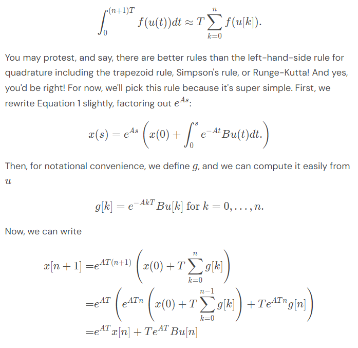
Now we have a really simple recurrence! We can compute it efficiently in the number of steps. This is a recurrent view, and we can use it to do fast inference like an RNN. Awesome!

---

1D: Convolutions

---

Part2: From Control Systems to Deep Learning

How do we apply this to deep learning? We'll build a new layer which is effectively a drop-in replacement for attention. Our goal will be to learn the A,B,C, matrices in the formulation. We want this process to be a) stable, b) efficient, and c) highly expressive. We'll take these in turn—but as we'll see they all have to do with the eigenvalues of A. In contrast, these properties are really difficult to understand for attention and took years of trial and error by a huge number of brilliant people. In S4, we're leveraging a bunch of brilliant people who worked this out while making satellites and cell phones.

---

2A: Stable

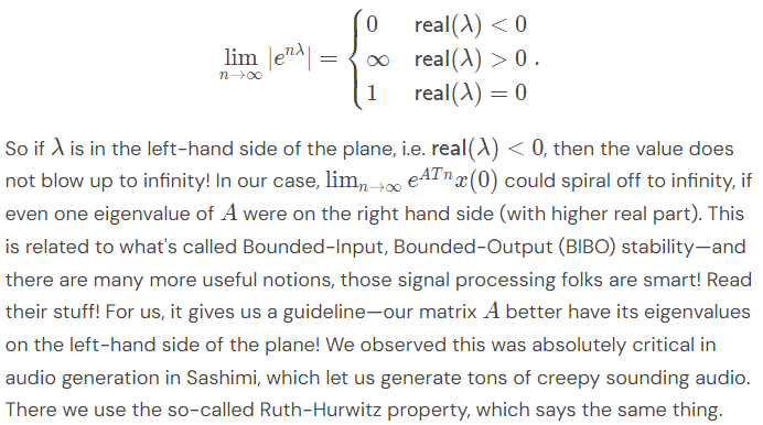
One thing that every electrical engineer knows is "keep your roots on the left-hand side of the plane." They may not know why they know it, but they know it. In our case, those roots are the same as the eigenvalues of A (if you're an electrical engineer, they actually are the roots of what's called the transfer function, which is the Laplace transform of our differential equation). If you're not an electrical engineer, this condition is for a pragmatic, simple reason. Recall that for a complex number λ:

---

2B: Efficient

We'll give two observations. First, as we'll see, for a powerful reason it suffices to consider diagonal matrices. This simplifies the presentation, but it's not essential to scalability—in fact, Hippo showed you could do this for many non-diagonal matrices. Second, we'll show how to compute the output (y[k]) without materializing the the hidden state (x[k]), which will make us much faster when we do batched learning. The speed up is linear in the size of the batch—this makes a huge difference in training time!

---

Diagonal Matrices

Here, we make a pair of observations that almost help us:

• If A were symmetric, then A would have a full set of real-valued eigenvalues, and it could be diagonalized by a linear (orthogonal) transformation.
• Since this module is a drop-in replacement for attention, the inputs (and the output) are multiplied by fully-connected layers. These models are capable of learning any change of basis transformation.

Combining these two observations, we could let A be real diagonal matrices and let the fully connected layer learn the basis—which would be super fast! We tried this, and it didn't work... so why not?

 

We learned that to obtain high quality the A matrix often had to be non-symmetric (non-hermitian) — so it didn't have real eigenvalues. At first blush, this seems to mean that we need to learn a general representation for A, but all is not lost. Something slightly weaker holds:

We can again compute this using our rectangle or convolution method—and life is good!

---

Even Faster! No Hidden State!

In many of our applications, we don't care about the hidden state—we just want the output of the layer, which recall is given by the state space equation:

Code Snippet These optimizations lead to a very concise forward pass (being a little imprecise about the shapes):

---

2C: Highly-Expressive Initialization

 

 

Thus, choosing k in this way effectively defines a decent basis.

 

For both of these, there are surely more clever things to do, but it seems to work ok!

---

Wrapping Up

Now that we've gone over the derivation, you can see it in action here. The entire kernel takes less than 100 lines of PyTorch code (even with some extra functionality from the Appendix that we haven't covered yet).

 

We saw that applying LTI systems to deep learning, we were able to use this theory to understand how to make these models stable, efficient, and expressive. One interesting aspect of these systems we inherent is that they are continuous systems that are discretized. This is really natural in physical systems, but hasn't been typical in machine learning until recently. We think this could open up a huge number of possibilities in machine learning. There are many improvements people have made in signal processing to discretize more faithfully, handle noise, and deal with structure. Perhaps those will be equally amazing in deep learning applications! We hope so.

 

We didn't cover some important standard extensions from our transformer and convolutional models—it's a drop in replacement for these models. This is totally standard stuff, and we include it just so you can get OK results.

• Many Filters, heads or SSMs: We don't train a single SSM per layer—we often train many more (say 256 of them). This is analogous to heads in attention or filters in convolutions.
• Nonlinearities: As is typical in both models, we have a non-linear fully connected layer (an FFN) that is responsible for mixing the features—note that it operates across filters—but not across the sequence length because that would be too expensive in many of our intended applications.

---

Appendix: Signal Processing Zero-Order Hold